Empirical Project 7 Solutions
These are not model answers. They are provided to help students, including those doing the project outside a formal class, to check their progress while working through the questions using the Excel, R, or Google Sheets walk-throughs. There are also brief notes for the more interpretive questions. Students taking courses using Doing Economics should follow the guidance of their instructors.
Part 7.1 Drawing supply and demand diagrams
- Solution figure 7.1 shows the two new variables and the actual values of P and Q.
| Year | log (Q) | log (P) | Q | P |
|---|---|---|---|---|
| 1930 | 4.45 | 4.76 | 85.51 | 116.95 |
| 1931 | 4.36 | 4.61 | 77.99 | 100.93 |
| 1932 | 4.20 | 4.37 | 66.99 | 78.89 |
| 1933 | 4.03 | 4.53 | 56.37 | 92.90 |
| 1934 | 4.10 | 4.64 | 60.12 | 104.00 |
| 1935 | 4.20 | 4.56 | 66.38 | 95.94 |
| 1936 | 4.14 | 4.85 | 62.52 | 127.94 |
| 1937 | 4.26 | 4.66 | 70.96 | 105.93 |
| 1938 | 4.26 | 4.69 | 70.80 | 108.90 |
| 1939 | 4.14 | 4.78 | 63.10 | 118.85 |
| 1940 | 4.35 | 4.69 | 77.09 | 108.90 |
| 1941 | 4.17 | 4.90 | 64.42 | 133.97 |
| 1942 | 4.03 | 5.48 | 56.50 | 239.89 |
| 1943 | 3.88 | 6.10 | 48.53 | 444.65 |
| 1944 | 4.26 | 5.91 | 70.80 | 368.14 |
| 1945 | 4.29 | 6.02 | 72.95 | 410.22 |
| 1946 | 4.39 | 5.95 | 80.91 | 383.72 |
| 1947 | 4.40 | 5.77 | 81.10 | 319.17 |
| 1948 | 4.30 | 5.96 | 73.79 | 389.06 |
| 1949 | 4.36 | 5.74 | 78.35 | 311.90 |
| 1950 | 4.41 | 5.78 | 82.42 | 322.86 |
| 1951 | 4.42 | 5.91 | 83.37 | 368.99 |
Prices and quantities of watermelons (values rounded to two decimal places).
Solution figure 7.1 Prices and quantities of watermelons (values rounded to two decimal places).
- Solution figures 7.2 and 7.3 provide line charts for P and Q.
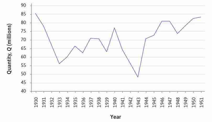
Price of watermelons (USD per 1,000, 1931–1950).
Solution figure 7.2 Price of watermelons (USD per 1,000, 1931–1950).
- Solution figure 7.4 provides the solution, with the solutions to (b) and (c).
- Solution figure 7.4 provides the solution, with the solutions to (a) and (c).
- Solution figure 7.4 provides the solution, with the solutions to (a) and (b).
| Q | Log Q | Supply (log P) | Demand (log P) | Supply (P) | Demand (P) |
|---|---|---|---|---|---|
| 20 | 3.00 | 3.09 | 6.04 | 22.04 | 421.37 |
| 25 | 3.22 | 3.47 | 5.86 | 32.20 | 350.91 |
| 30 | 3.40 | 3.78 | 5.71 | 43.91 | 302.18 |
| 35 | 3.56 | 4.04 | 5.58 | 57.06 | 266.30 |
| 40 | 3.69 | 4.27 | 5.48 | 71.60 | 238.68 |
| 45 | 3.81 | 4.47 | 5.38 | 87.47 | 216.70 |
| 50 | 3.91 | 4.65 | 5.29 | 104.63 | 198.77 |
| 55 | 4.01 | 4.81 | 5.21 | 123.03 | 183.83 |
| 60 | 4.09 | 4.96 | 5.14 | 142.65 | 171.17 |
| 65 | 4.17 | 5.10 | 5.08 | 163.44 | 160.29 |
| 70 | 4.25 | 5.22 | 5.02 | 185.39 | 150.84 |
| 75 | 4.32 | 5.34 | 4.96 | 208.46 | 142.55 |
| 80 | 4.38 | 5.45 | 4.91 | 232.63 | 135.20 |
| 85 | 4.44 | 5.55 | 4.86 | 257.88 | 128.64 |
| 90 | 4.50 | 5.65 | 4.81 | 284.20 | 122.75 |
| 95 | 4.55 | 5.74 | 4.77 | 311.56 | 117.43 |
| 100 | 4.61 | 5.83 | 4.72 | 339.95 | 112.59 |
Calculated prices and quantities (in natural logs and actual values).
Solution figure 7.4 Calculated prices and quantities (in natural logs and actual values).
- Solution figure 7.5 shows plotted supply and demand curves.
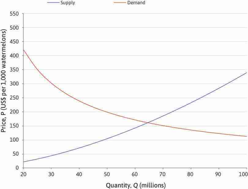
Supply and demand diagram.
Solution figure 7.5 Supply and demand diagram.
- Solution figure 7.5 provides the full table with columns added for ‘New supply (log P)’ and ‘New supply (P)’.
| Q | Log Q | Supply (log P) | Demand (log P) | Supply (P) | Demand (P) | New supply (log P) | New supply (P) |
|---|---|---|---|---|---|---|---|
| 20 | 3.00 | 3.09 | 6.04 | 22.04 | 421.37 | 3.49 | 32.88 |
| 25 | 3.22 | 3.47 | 5.86 | 32.20 | 350.91 | 3.87 | 48.04 |
| 30 | 3.40 | 3.78 | 5.71 | 43.91 | 302.18 | 4.18 | 65.50 |
| 35 | 3.56 | 4.04 | 5.58 | 57.06 | 266.30 | 4.44 | 85.12 |
| 40 | 3.69 | 4.27 | 5.48 | 71.60 | 238.68 | 4.67 | 106.81 |
| 45 | 3.81 | 4.47 | 5.38 | 87.47 | 216.70 | 4.87 | 130.49 |
| 50 | 3.91 | 4.65 | 5.29 | 104.63 | 198.77 | 5.05 | 156.09 |
| 55 | 4.01 | 4.81 | 5.21 | 123.03 | 183.83 | 5.21 | 183.55 |
| 60 | 4.09 | 4.96 | 5.14 | 142.65 | 171.17 | 5.36 | 212.81 |
| 65 | 4.17 | 5.10 | 5.08 | 163.44 | 160.29 | 5.50 | 243.83 |
| 70 | 4.25 | 5.22 | 5.02 | 185.39 | 150.84 | 5.62 | 276.56 |
| 75 | 4.32 | 5.34 | 4.96 | 208.46 | 142.55 | 5.74 | 310.98 |
| 80 | 4.38 | 5.45 | 4.91 | 232.63 | 135.20 | 5.85 | 347.04 |
| 85 | 4.44 | 5.55 | 4.86 | 257.88 | 128.64 | 5.95 | 384.72 |
| 90 | 4.50 | 5.65 | 4.81 | 284.20 | 122.75 | 6.05 | 423.98 |
| 95 | 4.55 | 5.74 | 4.77 | 311.56 | 117.43 | 6.14 | 464.79 |
| 100 | 4.61 | 5.83 | 4.72 | 339.95 | 112.59 | 6.23 | 507.14 |
New supply after the shock.
Solution figure 7.6 New supply after the shock.
- Solution figure 7.7 shows the line chart with the additional New supply (P) values plotted.
- From Solution figure 7.7, we can see that total surplus, producer surplus, and consumer surplus have all decreased.
Part 7.2 Interpreting supply and demand curves
- We rewrite the supply equation as log Q = 1.18 + 0.59 log P. The price elasticity of supply is therefore 0.59, which is inelastic (so supply is not very responsive to changes in price).
- The demand equation can be written as log Q = 10.37 – 1.22 log P. The price elasticity of demand is therefore 1.22, which is elastic (demand is relatively responsive to changes in price).
Note: This data exercise highlights why it is necessary to calculate the elasticities of supply and demand from the data rather than simply looking at the shapes of the supply and demand curves as they appear with the chosen scales for the horizontal and vertical axes.
- Economic interpretation and elasticity (where relevant) of given coefficients:
- Price of watermelons: The coefficient is positive, meaning that farmers supply more when the price is higher. The (own) price elasticity of supply is 0.58 and this coefficient is estimated quite precisely (small confidence interval), so we can conclude that supply is price inelastic.
- Price of cotton; price of vegetables: The coefficient represents the cross-price elasticity of supply (how responsive supply is to the price of other goods). The coefficient is negative. Cotton and vegetables are alternative crops to plant instead of watermelons, so when they become more expensive, farmers will produce fewer watermelons and produce cotton/vegetables instead. The cross-price elasticities of supply are both smaller than 1 (in absolute value) and quite precisely estimated, so we can conclude that watermelon supply is not very responsive to the prices of cotton and vegetables.
- Cotton program: This program was intended to limit production of cotton (one alternative crop to watermelons). The coefficient is positive and precisely estimated, so we can be quite confident that the policy resulted in some land being dedicated to watermelon production instead.
- Second World War: This event was a negative supply shock, because some land was dedicated to the war effort instead of watermelon production. The coefficient is negative and quite precisely estimated, so we can conclude that the war did have the effect of reducing supply.
- Economic interpretation and elasticity (where relevant) of given coefficients:
- Price of watermelons: The own-price elasticity is negative (as expected), but since the confidence intervals are quite wide, we cannot make any conclusions about how responsive demand is to price.
- Per-capita income: Per-capita demand for watermelons increases with income, but again, the confidence intervals are quite wide so we do not have a precise estimate of the income elasticity of demand.
- Railway freight costs: The coefficient is negative, meaning that demand decreases as transportation costs increase (as expected). The 95% confidence interval is quite wide so we do not have a precise estimate of how responsive demand is to railway freight costs.
- Many possible examples, including:
- A sudden change in consumers’ preferences for watermelon: If a medical article is published that extols the benefits of eating watermelons, watermelons may suddenly become a trendy diet food and the demand curve would shift to the right.
- Demand-side policy changes: A government health initiative that involves subsidies for purchasing any type of fruits would increase the demand for watermelons, shifting the demand curve to the right.
