Empirical Project 9 Working in Google Sheets
Google Sheets-specific learning objectives
In addition to the learning objectives for this project, in this section you will learn how to create and format time variables.
Part 9.1 Households that did not get a loan
Learning objectives for this part
- identify credit-constrained and credit-excluded households using survey information
- create dummy (indicator) variables
- compare characteristics of successful borrowers, discouraged borrowers, credit-constrained households, and credit-excluded households
- explain why selection bias is an important issue.
The Ethiopian Socioeconomic Survey (ESS) data was collected in 2013–14 from a nationally representative sample of households. Households were asked about topics such as their housing conditions, assets, and access to credit.
Download the ESS data and survey questionnaire:
- Download the ESS data. The Excel file contains three tabs (‘Data dictionary’, ‘All households’, and ‘Got loan’). Read the Data dictionary tab and make sure you know what each variable represents. (Later we will discuss exactly how some of these variables were constructed.)
- For the documentation, go to the data download site. Click on the ‘Documentation’ tab in the middle of the page.
- Under the heading ‘Questionnaires’, download the PDF file called ‘2013–2014 Ethiopian Socioeconomic Survey, Household Questionnaire’ by clicking the ‘Download’ button on the right-hand side of the page. You may find it helpful to refer to Section 14 of the questionnaire for the exact questions asked about credit and saving.
- The data is already in a format clean enough to use, so we will begin by summarizing the information in the ‘All households’ tab, starting with region and household characteristics.
- Create a pivot table showing the proportion of households that lived in each region and area type, with ‘region’ as the row variable and ‘rural’ as the column variable. (For help on creating pivot tables, see Google Sheets walk-through 3.1.)
- dummy variable (indicator variable)
- A variable that takes the value 1 if a certain condition is met, and 0 otherwise.
- Use Google Sheets’ IF function to create a variable that equals 1 if the household head was female, and 0 if the household head was male. Variables that are coded in this way are known as dummy variables (or indicator variables). What percentage of household heads were female?
- Create an appropriate summary table for the variables ‘hhsize’, ‘gender’, ‘age’, ‘young_children’, ‘working_age_adults’, ‘max_education’, and ‘number_assets’. (You may find it helpful to refer to Figure 2.9 in Empirical Project 2 for one possible format to use.)
- Write a short paragraph describing the information in your tables for 1(c).
Now that we have an idea of what our data looks like, we will move on to identify households that are potentially excluded from the credit market or are credit constrained. The former are households who find it impossible to borrow and the latter are households who can only borrow on unfavourable terms (see Section 9.10 of Economy, Society, and Public Policy).
The variables in our dataset that are related to this issue are ‘did_not_apply’ and ‘loan_rejected’. We will soon also look at the responses given in the variables ‘reason_not_apply1’ and ‘reason_not_apply2’.
- Using the ‘All households’ tab:
- Create a frequency table with ‘did_not_apply’ as the row variable and ‘loan_rejected’ as the column variable. Include the blanks as a separate row.
- Looking at these two variables, explain why some observations should be excluded and remove them from the dataset. Also remove all households with missing information for one or more of these variables. Of the non-excluded observations, what percentage of households applied for a loan over the past 12 months? Of those households, what percentage were successful?
- For the resulting categories in the frequency table, explain whether the households in that category can be described as credit constrained, credit excluded, or both.
To create operational categories to use throughout this project, we will label households as either:
- ‘successful’: households that applied for a loan and were given the loan
- ‘denied’: households that applied but were not given the loan
- ‘did not apply’: households that did not apply for a loan.
You should note that the ‘denied’ households are only a subset of the credit-excluded households as there will be households that are credit excluded and do not even apply for a loan. One could, for instance, reason that households who answered ‘Inadequate Collateral’ or ‘Do Not Know Any Lender’ are also likely to be credit excluded.
- Using the subset of data from Question 2(b):
- Create a new variable called ‘HH_status’ with the above categories.
- Create a new variable ‘discouraged_borrower’ that takes the value 1 if the household did not apply for a loan because it believed that it would not receive a loan (answered ‘Believe Would Be Refused’ in ‘reason_not_apply1’ or ‘reason_not_apply2’). How many households (and what percentage) are discouraged borrowers? (Note: this is a fairly narrow definition of ‘discouraged’ and one could easily argue that other criteria should also be considered under this label.)
Note that arguably other answers are also indicative of being credit constrained, and so the criteria we use is definitely only a subset of all households that are credit constrained. For example, one could include households that have been denied a loan, and it is also indeed likely that some households that have been granted a loan are in fact credit constrained.
- Create a new variable ‘credit_constrained’ that takes the value 1 (or yes) for households that gave a reason for not applying other than ‘NA’, ‘Other’, or ‘Have Adequate Farm’ in either of the two questions ‘reason_not_apply1’ or ‘reason_not_apply2’, and 0 otherwise. For example, a household that answers ‘Have Adequate Farm’ in ‘reason_not_apply1’ and ‘Do Not Know Any Lender’ would not be classified as credit constrained. How many households (and what percentage) are credit constrained?
- Create a frequency table showing the most important reason for not applying for a loan, and another showing the second most important reason for not applying. What were the most common reasons for not applying?
We will now analyse the stated reasons for wanting a loan, comparing those households that were successful (‘HH_status’ equal to ‘successful’) with those that were not successful (‘HH_status’ equal to ‘denied’).
- For both groups, create one table showing the proportion of households for each loan purpose. (You will realize that in the ‘All households’ tab, the reason for all successful loans is ‘Other’. For that reason, you should use the ‘Got loan’ tab to retrieve the reasons for loan information for successful loans.) Was the purpose of loans for denied and successful borrowers similar? (Hint: It may help to think about the broad categories of spending on consumption and investment).
- Using the information in the ‘All households’ tab and ‘Got loan’ tab, for each group of households:
- Create a table as shown in Figure 9.1 to compare the averages of the specified household characteristics.
| Household characteristic | Successful | Denied |
|---|---|---|
| Age of household head | ||
| Highest education in household | ||
| Number of assets | ||
| Household size | ||
| Number of young children | ||
| Number of working-age adults |
Characteristics of successful and denied borrowers.
Figure 9.1 Characteristics of successful and denied borrowers.
- For each characteristic, explain how it may affect a household’s ability to get a loan (ceteris paribus).
- Looking at your table from Question 5(a), discuss whether you see this pattern in the data. (For example, are successful borrowers older/younger on average than denied borrowers?)
- conditional mean
- An average of a variable, taken over a subgroup of observations that satisfy certain conditions, rather than all observations.
- Now try conditioning on the variable ‘rural’ or ‘region’ and discuss how (if at all) your results change.
- Using Figure 9.1, without conditioning on ‘rural’ or ‘region’, carry out the following:
- Calculate the difference in means (‘successful’ borrowers minus ‘denied’ borrowers).
- Calculate the 95% confidence interval for the difference in means between the two subgroups (‘successful’ minus ‘denied’). (Hint: Use Google Sheets’ CONFIDENCE.T function and see Part 8.3 of Empirical Project 8 for help on how to do this.)
- Plot a column chart showing the differences on the vertical axis (sorted from smallest to largest), and household characteristics on the horizontal axis. Add the confidence intervals from Question 6(b) to the chart.
- Interpret your findings.
- Using the information in the ‘All households’ tab:
- Create a table similar to Figure 9.1, but with additional columns for discouraged borrowers and credit-constrained households.
- Compare the means across the four groups and discuss any similarities/differences you observe (you do not need to do any formal calculations).
- selection bias
- An issue that occurs when the sample or data observed is not representative of the population of interest. For example, individuals with certain characteristics may be more likely to be part of the sample observed (such as students being more likely than CEOs to participate in computer lab experiments).
A study on access to loans in Ethiopia looked at the relationship between loan amount and household characteristics. When doing so, they needed to account for selection bias, because we only observe positive loan amounts for successful borrowers. If we only had data for successful borrowers, then our sample would not be representative of the population of interest (all households), so we would have to interpret our results with caution. In our case, we have information about all households, so we can compare observable characteristics to see whether successful borrowers are similar to other households.
An article by the Institute for Work and Health explains selection bias in more detail, and why it is a problem encountered by all areas of research.
- Think of another example where there might be selection bias, in other words, where the data we observe is not representative of the population of interest.
Part 9.2 Households that got a loan
Learning objectives for this part
- analyse the characteristics of loans obtained by successful borrowers.
For households that successfully got a loan, we will look at:
- purpose of the loan
- duration of the loan(s)
- loan amount and interest rate charged
- who the household borrowed from.
We will also see if there are any relationships between these loan characteristics and household characteristics.
Now we will use the variables relating to the loan start and end dates to calculate the duration of the loan. Before using these variables, we need to check that the variable entries make sense. Some of this information could be recorded incorrectly (for example, the year is missing a digit, or the month is a number rather than a word).
- Using the ‘Got loan’ tab, do the following:
- Check the variables ‘loan_startmonth’, ‘loan_startyear’, ‘loan_endmonth’, and ‘loan_endyear’ and replace the entries that are recorded incorrectly with either the correct entry (if possible), or as blank (if not possible to infer the correct entry). (Note: Some entries are recorded as ‘Pagume’, which corresponds to early September in the Ethiopian calendar.)
- To calculate loan duration, we need to combine the month and year variables into one date variable. Use Google Sheets’ CONCATENATE function to create new variables for the start and end date, and format them as date variables. (See Google Sheets walk-through 9.1 for help on how to do this.)
- Some of the dates (months or years) are missing. Calculate the percentage of the data that is missing and explain whether you think missing data is a serious problem.
- Create a new variable containing the loan duration (end date minus start date), which will be measured in days.
- You will notice that some dates were recorded incorrectly, with the start date later than the end date. We could either treat these entries as missing or swap the start and end dates. Create two new variables for loan duration, one with all negative entries recorded as blank, and one with negative entries replaced as positive numbers. (Hint: Google Sheets’ ABS function converts any number to a positive number.)
- For this project we will define a long-term loan as lasting more than a year (365 days), which we will use in later questions. For this definition use the loan length variable that converts negative loan lengths to positive ones. Create an indicator variable called ‘long_term’ that equals 1 if the loan was long term, and 0 otherwise. What percentage of loans were long term?
Google Sheets walk-through 9.1 Creating and formatting time variables
The data
In this example, we will use the month and year variables in Columns O, P, R, and S to make new date variables in Columns V and W. Before doing this, we need to make sure all the months and years are coded correctly, otherwise Google Sheets may not recognize these values as dates. Also, some cells are blank, so we need to make our cell formulas work regardless of missing data.
Figure 9.2a In this example, we will use the month and year variables in Columns O, P, R, and S to make new date variables in Columns V and W. Before doing this, we need to make sure all the months and years are coded correctly, otherwise Google Sheets may not recognize these values as dates. Also, some cells are blank, so we need to make our cell formulas work regardless of missing data.
Combine the month and year variables into one variable
The CONCATENATE function combines text in cells in the specified order. You can add punctuation and spaces by specifying them in quotation marks (“”). Here, we use the IF function so that Google Sheets only fills in cells in rows where both start and end dates were non-missing (the AND function states these conditions).
Figure 9.2b The CONCATENATE function combines text in cells in the specified order. You can add punctuation and spaces by specifying them in quotation marks (“”). Here, we use the IF function so that Google Sheets only fills in cells in rows where both start and end dates were non-missing (the AND function states these conditions).
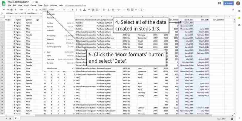
Reformat the cells as date variables
After step 5, you may not notice any visible changes to the text in cells, but Google Sheets now recognizes them as dates and you can use them to make calculations, such as counting the number of days between two dates.
Figure 9.2c After step 5, you may not notice any visible changes to the text in cells, but Google Sheets now recognizes them as dates and you can use them to make calculations, such as counting the number of days between two dates.
Use date variables to calculate duration
With the proper formatting, Google Sheets can calculate the number of days between two dates. In this example, some of the start dates are later than the end dates, resulting in negative numbers. We will correct these values in the next step.
Figure 9.2d With the proper formatting, Google Sheets can calculate the number of days between two dates. In this example, some of the start dates are later than the end dates, resulting in negative numbers. We will correct these values in the next step.
Recode incorrect durations
The ABS function converts any value to its positive counterpart. After step 9, the negative values in Column X are now recorded as positive numbers in Column Y. Again, we used the AND function so that Google Sheets only did this for non-blank cells (in this case, the condition AND(X2<>“”) would give the same results).
Figure 9.2e The ABS function converts any value to its positive counterpart. After step 9, the negative values in Column X are now recorded as positive numbers in Column Y. Again, we used the AND function so that Google Sheets only did this for non-blank cells (in this case, the condition AND(X2<>“”) would give the same results).
- Using the variables ‘loan_amount’ and ‘loan_interest’:
- Create summary tables to summarize the distribution of loan amount (mean, standard deviation, maximum, and minimum), one using the loan amount, the other using the total amount to repay (loan amount + interest). Make sure to exclude the one observation previously identified as having an extremely high interest rate. Remember to give your tables meaningful titles. Describe any features of the data that you find interesting.
- As mentioned earlier, the interest rate is a borrowing condition that can vary widely across households. Here we will take the interest rate to be the interest paid as a percentage of the loan amount. Calculate the interest rate for each loan in the data. (Exclude observations where the interest paid is not recorded.)
- Check for extreme values (interest rates that are either very large or zero). You may also want to create a scatterplot (with interest rate on the vertical axis and loan amount on the horizontal axis) to help you identify extreme (atypical) observations. Exclude the observation with the most extreme interest rate from further calculations. What percentage of the loans are zero interest?
- Make summary tables of the mean, maximum, minimum, and quartiles of the loan amount and interest rate, calculating these measures separately for long-term and short-term loans. Compare the distributions of interest rates for short-term and long-term loans.
- Create a table showing the correlation between the interest rate and household characteristics (you may want to refer to Figure 8.6 in Empirical Project 8 for an example). Interpreting the interest rate charged as a measure of default risk (inability to repay), explain whether the relationships implied by the coefficients are what you expected (for example, would you expect interest rates to be higher for households with less assets, more dependents etc.).
For help on making scatterplots and calculating correlation coefficients, see Google Sheets walk-through 1.7.
- Now we will look at sources of finance and how they are related to loan characteristics.
- Create a table showing the proportion of loans (in terms of the column variable) with source of finance (‘borrowed_from’) as the row variable and ‘rural’ as the column variable. Make a similar table but with ‘borrowed_from_other’ as the row variable instead. Does it look like rural households use different sources of finance from urban households? (Hint: It may help to think about sources of finance in terms of formal, informal, and other institutions such as microfinancers or NGOs.)
-
For each of the variables below, create a table showing the average of that variable, with ‘borrowed_from’ as the row variable and ‘rural’ as the column variable. Comment on any similarities or differences between rows and columns that you find interesting, and suggest explanations for what you observe.
- duration of loan (using the variable in which negative durations were transformed to positive durations)
- loan amount
- interest rate
- Create a table showing the proportion of ‘gender’ (in terms of the row variable) with ‘borrowed_from’ as the row variable and ‘rural’ as the column variable. Describe any relationships you observe between the gender of household head, the place where he/she lives, and the types of finance used.
- What other variables are currently not in our dataset but could also be important for our analysis in Questions 2 and 3?
- In this project we have looked at patterns in borrowing and access to credit, but we are not able to make any causal statements such as ‘changes in X will cause households to be credit constrained’ or ‘characteristic Y causes improved access to credit’. Outline a policy intervention that could help improve households’ access to loans, and how to design the implementation so you can assess the causal effects of this policy.
