Empirical Project 9 Working in R
Download the code
To download the code chunks used in this project, right-click on the download link and select ‘Save Link As…’. You’ll need to save the code download to your working directory, and open it in RStudio.
Don’t forget to also download the data into your working directory by following the steps in this project.
Getting started in R
For this project you will need the following packages:
-
tidyverse, to help with data manipulation -
readxl, to import an Excel spreadsheet -
knitr, to format tables -
mosaic, to help create frequency tables.
If you need to install these packages, run the following code:
install.packages(c("readxl", "tidyverse", "knitr", "mosaic"))
You can import the libraries now, or when they are used in the R walk-throughs below.
library(readxl)
library(tidyverse)
library(knitr)
library(mosaic)
Part 9.1 Households that did not get a loan
Learning objectives for this part
- identify credit-constrained and credit-excluded households using survey information
- create dummy (indicator) variables
- compare characteristics of successful borrowers, discouraged borrowers, credit-constrained households, and credit-excluded households
- explain why selection bias is an important issue.
The Ethiopian Socioeconomic Survey (ESS) data was collected in 2013–14 from a nationally representative sample of households. Households were asked about topics such as their housing conditions, assets, and access to credit.
Download the ESS data and survey questionnaire:
- Download the ESS data. The Excel file contains three tabs (‘Data dictionary’, ‘All households’, and ‘Got loan’). Read the ‘Data dictionary’ tab and make sure you know what each variable represents. For Part 9.1 we will use the data from the ‘All households’ tab. The ‘Got loan’ data will be used in Part 9.2.
- For the documentation, go to the data download site. Click on the ‘Documentation’ tab in the middle of the page.
- Under the heading ‘Questionnaires’, download the PDF file called ‘2013–2014 Ethiopian Socioeconomic Survey, Household Questionnaire’ by clicking the ‘Download’ button on the right-hand side of the page. You may find it helpful to refer to Section 14 of the questionnaire for the exact questions asked about credit and saving.
R walk-through 9.1 Importing data into R
Before importing the data, open it in Excel to look at its structure. You can see there are three tabs: ‘Data dictionary’, ‘All households’, and ‘Got loan’. We will import them into separate dataframes (
DataDict,allHH, andgotLrespectively). We import the ‘Data dictionary’ so that we do not have to return to the Excel spreadsheet.Also note that there are a lot of empty cells, which is how missing data is coded in Excel (but not in R). In the
read_excelfunction we therefore use thena = ""option so that R recognizes empty cells as missing data.library(tidyverse) library(readxl) # Set your working directory to the correct folder. # Insert your file path for 'YOURFILEPATH'. setwd("YOURFILEPATH") allHH read_excel("Project 9 datafile.xlsx", sheet = "All households", na = "NA") gotL read_excel("Project 9 datafile.xlsx", sheet = "Got loan", na = "NA") DataDict read_excel("Project 9 datafile.xlsx", sheet = "Data dictionary", na = "NA")Now let’s look at the variable types for
allHHandgotL. To see the variable definitions, use the commandview(DataDict).str(allHH)## Classes 'tbl_df', 'tbl' and 'data.frame': 5262 obs. of 19 variables: ## $ household_id2 : num 1.01e+16 1.01e+16 1.01e+16 1.01e+16 1.01e+16 ... ## $ got_loan : chr "No" "No" "No" "Yes" ... ## $ rural : chr "Rural" "Rural" "Rural" "Rural" ... ## $ hhsize : num 8 8 1 3 4 4 5 5 6 7 ... ## $ region : chr "Tigray" "Tigray" "Tigray" "Tigray" ... ## $ gender : chr "Female" "Male" "Female" "Female" ... ## $ age : num 78 37 78 30 71 28 37 32 51 43 ... ## $ young_children : num 4 5 0 1 1 3 2 3 3 2 ... ## $ working_age_adults: num 3 3 0 2 1 1 3 2 3 6 ... ## $ max_education : num 3 0 0 4 8 4 9 6 4 5 ... ## $ number_assets : num 32 19 3 6 34 5 45 35 20 64 ... ## $ loan_rejected : chr "No" "No" "No" "No" ... ## $ rejection_source1 : chr NA NA NA NA ... ## $ rejection_source2 : chr NA NA NA NA ... ## $ loan_purpose : chr NA NA NA NA ... ## $ loan_purpose_other: chr NA NA NA NA ... ## $ did_not_apply : chr "Did not apply" "Did not apply" "Did not apply" "Applied" ... ## $ reason_not_apply1 : chr "Too Expensive" "Believe Would Be Refused" "Too Expensive" NA ... ## $ reason_not_apply2 : chr "Fear Not Be Able To Pay" NA "Fear Not Be Able To Pay" NA ...str(gotL)## Classes 'tbl_df', 'tbl' and 'data.frame': 1480 obs. of 21 variables: ## $ household_id2 : num 1.01e+16 1.01e+16 1.01e+16 1.01e+16 1.01e+16 ... ## $ got_loan : chr "Yes" "Yes" "Yes" "Yes" ... ## $ rural : chr "Rural" "Rural" "Rural" "Rural" ... ## $ hhsize : num 3 4 5 9 7 7 8 7 10 8 ... ## $ region : chr "Tigray" "Tigray" "Tigray" "Tigray" ... ## $ gender : chr "Female" "Male" "Male" "Male" ... ## $ age : num 30 71 53 52 56 38 44 47 52 37 ... ## $ young_children : num 1 1 3 4 3 4 4 3 2 6 ... ## $ working_age_adults : num 2 1 2 6 3 3 4 4 8 2 ... ## $ max_education : num 4 8 5 8 7 7 8 6 10 1 ... ## $ number_assets : num 6 34 14 16 9 14 24 15 22 10 ... ## $ borrowed_from : chr "Relative" "Relative" "Relative" "Other (specify)" ... ## $ borrowed_from_other: chr NA NA NA "Cooperatives" ... ## $ loan_purpose : chr "Purchase Agricultural Inputs for Food Crop" "Purchase Agricultural Inputs for Food Crop" "Purchase Agricultural Inputs for Food Crop" "Purchase Agricultural Inputs for Food Crop" ... ## $ loan_startmonth : chr "March" "November" "November" "June" ... ## $ loan_startyear : num 2004 2006 2006 2005 2005 ... ## $ loan_repaid : chr "Yes" "Yes" "No" "No" ... ## $ loan_endmonth : chr NA NA "June" "March" ... ## $ loan_endyear : num NA NA 2006 2006 2006 ... ## $ loan_amount : num 1000 800 2500 2653 1600 ... ## $ loan_interest : num 300 0 1750 325 300 1750 290 300 300 268 ...It is important to ensure that all variables we expect to be numerical (numbers) are coded as
num, and in this case, they are. You can see that there are many variables that are coded as character (chr) variables because they are text (for examplegenderorregion), but since we can use these variables to group data by category, we will useas.factorto change them into categorical (factor) variables for later use.Instead of converting each character variable to a factor variable individually, say
allHH$gender as.factor(allHH$gender), we use the piping operator (%>%) from thetidyversepackage to do this step in one go. (For a more detailed introduction to piping, see the University of Manchester’s Econometric Computing Learning Resource).We take
allHHand use themutate_iffunction, which applies theas.factorfunction to character variables only. Then we do the same forgotL.allHH allHH %>% mutate_if(is.character, as.factor) gotL gotL %>% mutate_if(is.character, as.factor)Typing
str(allHH)andstr(gotL)will confirm that all character variables are now categorical variables.
- The data is already in a format clean enough to use, so we will begin by summarizing the information in the ‘All households’ tab, starting with region and household characteristics.
- Create a table showing the proportion of households that lived in each region and area type, with
regionas the row variable andruralas the column variable. (For help on creating tables, see R walk-through 3.3.)
- Use the
Gendervariable to find what percentage of household heads were female.
- Create an appropriate summary table for the variables
hhsize,gender,age,young_children,working_age_adults,max_education, andnumber_assets. (You may find it helpful to refer to R walk-through 2.7 in Empirical Project 2 for one possible format to use.)
- Write a short paragraph describing the information in your tables for 1(c).
R walk-through 9.2 Creating summary tables
In order to get the proportions of households living in large towns, small towns, or rural areas (encoded in the variable
rural), we use thetablefunction. The counts (number) of households in the respective regions and area types are contained in stab1. Running this table through theprop.table()function changes the values from counts to proportions. The optional input(, 1)makes the proportions for each row add to one. (You could see what happens when you leave this option out, or if you choose the value2.) To obtain detailed information, use the command?prop.table .# Control how many digits are printed options(digits = 3) stab1 table(allHH$region, allHH$rural) prop.table(stab1, 1)## ## Large town (urban) Rural Small town (urban) ## Addis Ababa 1.0000 0.0000 0.0000 ## Afar 0.0956 0.7574 0.1471 ## Amhara 0.2176 0.6692 0.1132 ## Benshagul Gumuz 0.0000 0.9040 0.0960 ## Diredwa 0.4685 0.5315 0.0000 ## Gambelia 0.1154 0.8000 0.0846 ## Harari 0.2727 0.7273 0.0000 ## Oromia 0.2831 0.6070 0.1098 ## SNNP 0.1826 0.7270 0.0905 ## Somalie 0.1552 0.7552 0.0897 ## Tigray 0.3670 0.5628 0.0701Let’s use a similar approach to calculate the percentage of households with female heads (encoded in the variable
gender).stab2 table(allHH$gender) prop.table(stab2)## ## Female Male ## 0.304 0.696As shown, 30.4% of households have a female head.
We need to provide summary statistics for a range of variables. Most of these variables are numeric variables, but one,
gender, is a factor variable. For the latter, we use thesummaryfunction. For the numeric variables we use thefavstatsfunction, which is part of themosaicpackage. We could also use thesummaryfunction, but it does not provide the standard deviations that we need.The summary statistics for the numeric variables are generated using the
lapply(list apply) function. Inside the function we specify the subset of variables we are interested in,subset(allHH, select = sel_q), and specify the function we want to apply to these variables, namely thefavstatsfunction.# Load the mosaic package library(mosaic) summary(allHH$gender)## Female Male NA's ## 1599 3662 1# Create a list of the numeric variable names sel_q c('hhsize', 'age', 'young_children', 'working_age_adults', 'max_education', 'number_assets') lapply(subset(allHH, select = sel_q), favstats)## $hhsize ## min Q1 median Q3 max mean sd n missing ## 1 3 4 6 16 4.58 2.4 5260 2 ## ## $age ## min Q1 median Q3 max mean sd n missing ## 3 32 42 55 99 44.2 15.6 5253 9 ## ## $young_children ## min Q1 median Q3 max mean sd n missing ## 0 0 2 3 10 1.89 1.71 5262 0 ## ## $working_age_adults ## min Q1 median Q3 max mean sd n missing ## 0 2 2 3 10 2.58 1.52 5262 0 ## ## $max_education ## min Q1 median Q3 max mean sd n missing ## 0 2 6 10 30 7.53 7.28 5262 0 ## ## $number_assets ## min Q1 median Q3 max mean sd n missing ## 0 5 9 18 203 14.9 17.2 5262 0
Now that we have an idea of what our data looks like, we will move on to identifying households that are potentially excluded from the credit market or are credit constrained. The former are households that find it impossible to borrow, and the latter are households that can only borrow on unfavourable terms (see Section 9.10 of Economy, Society, and Public Policy).
The variables in our dataset that are related to this issue are did_not_apply and loan_rejected. Later we will also look at the responses given in the variables ‘reason_not_apply1’ and ‘reason_not_apply2’.
- Using the ‘All households’ dataset:
- Create a frequency table with
did_not_applyas the row variable andloan_rejectedas the column variable. Include all ‘NA’ as a separate row.
- Looking at these two variables, explain why some observations should be excluded and remove them from the dataset. Also remove all households with missing information for one or more of these variables. Of the non-excluded observations, what percentage of households applied for a loan over the past 12 months? Of those households, what percentage were successful?
- For the resulting categories in the frequency table, explain whether the households in that category can be described as credit constrained, credit excluded, or both.
R walk-through 9.3 Making frequency tables for loan applications and outcomes
The easiest way to make a frequency table is to use the
tablefunction. Note that we nested thetable ()function in theaddmarginsfunction to obtain row and column totals.By default, the table function excludes missing (
NA) values. Consulting the help function (type?tablein the command window) will show that the optionuseNA = "always"includes these values.stab3 addmargins(table( allHH$did_not_apply, allHH$loan_rejected, useNA = "always", dnn = c("Applied?", "Rejected?"))) stab3## Rejected? ## Applied? No YesSum ## Applied 1363 201 1 1565 ## Did not apply 3632 24 2 3658 ##37 2 0 39 ## Sum 5032 227 3 5262Here, we decide to exclude the 24 households that indicated that they did not apply for a loan, but also indicated that they were refused a loan. This is a contestable decision, as it results in excluding more than 10% of households that indicated that they were refused a loan. We shall also remove all observations that have missing data for any of these two questions.
Now we create the dataset with the non-missing data only (
allHHc).# Remove NAs in did_not_apply allHHc subset(allHH, !is.na(allHH$did_not_apply)) allHHc subset(allHHc, !is.na(allHHc$loan_rejected)) # Show the number of observations nrow(allHHc)## [1] 5220At this stage we have dropped 42 observations. Now we delete the 24 observations that gave a nonsensical answer.
allHHc  subset(allHHc,
  !(allHHc$loan_rejected == "Yes" &
  allHHc$did_not_apply == "Did not apply"))

# Show the number of observations
nrow(allHHc)
## [1] 5196We are left with 5,196 observations. Let’s recreate the frequency table, but this time adding the
prop.tablefunction to calculate proportions. (To obtain percentages, multiply the proportions by 100.)stab4 addmargins(prop.table(table( allHHc$did_not_apply, allHHc$loan_rejected, dnn = c("Applied?", "Rejected?")))) stab4## Rejected? ## Applied? No Yes Sum ## Applied 0.2623 0.0387 0.3010 ## Did not apply 0.6990 0.0000 0.6990 ## Sum 0.9613 0.0387 1.0000
To create operational categories to use throughout this project, we will label households as either:
- ‘successful’: households that applied for a loan and were given the loan
- ‘denied’: households that applied but were not given the loan
- ‘did not apply’: households that did not apply for a loan.
You should note that the ‘denied’ households are only a subset of the credit-excluded households, as there will be households that are credit excluded and do not even apply for a loan. One could, for instance, reason that households who answered ‘Inadequate Collateral’ or ‘Do Not Know Any Lender’ are also likely to be credit excluded.
- Using the subset of data from Question 2(b):
- Create a new variable called
HH_statuswith the above categories.
- Create a new variable
discouraged_borrowerthat takes the value 1 if the household did not apply for a loan because it believed that it would not receive a loan (answered ‘Believe Would Be Refused’ inreason_not_apply1orreason_not_apply2). How many households (and what percentage) are discouraged borrowers? (Note: This is a fairly narrow definition of ‘discouraged’ and one could easily argue that other criteria should also be considered under this label.)
Note that arguably other answers are also indicative of being credit constrained, so the criteria we use is definitely only a subset of all households that are credit constrained. For example, one could include households that have been denied a loan, and it is also likely that some households that have been granted a loan are in fact credit constrained.
- Create a new variable
credit_constrainedthat takes the value 1 (or yes) for households that gave a reason for not applying other than ‘NA’, ‘Other’, or ‘Have Adequate Farm’ in either of the two questionsreason_not_apply1orreason_not_apply2, and 0 otherwise. For example, a household that answers ‘Have Adequate Farm’ inreason_not_apply1and ‘Do Not Know Any Lender’ would not be classified as credit constrained. How many households (and what percentage) are credit constrained?
- Create a frequency table showing the most important reason for not applying for a loan, and another showing the second most important reason for not applying. What were the most common reasons for not applying?
R walk-through 9.4 Creating variables to classify households
Let’s first create the
HH_statusvariable. We set the values ofHH_statusto”not applied”, then use logical indexing to change all entries where households applied for a loan (allHHc$did_not_apply == “Applied”) and were accepted (allHHC$loan_rejected == “No”) to“successful”, and households who were denied ((allHHC$loan_rejected == “Yes”) to”denied”.# This is the default category. allHHc$HH_status "not applied" allHHc$HH_status[allHHc$did_not_apply == "Applied" & allHHc$loan_rejected == "No"] "successful" allHHc$HH_status[allHHc$did_not_apply == "Applied" & allHHc$loan_rejected == "Yes"] "denied" # Change from character to factor variable allHHc$HH_status factor(allHHc$HH_status)Typing
summary(allHHc$HH_status)should give you numbers that correspond to the frequency table from Question 2.Let’s continue by using the same steps to make the
discouraged_borrowervariable.# This is the default category. allHHc$discouraged_borrower "No" allHHc$discouraged_borrower[allHHc$reason_not_apply1 == "Believe Would Be Refused"] "Yes" allHHc$discouraged_borrower[allHHc$reason_not_apply2 == "Believe Would Be Refused"] "Yes" # Change from character to factor variable allHHc$discouraged_borrower factor(allHHc$discouraged_borrower) summary(allHHc$discouraged_borrower)## No Yes ## 4608 588To make the
credit_constrainedvariable, we use thelevelsfunction to check all the possible answers to thereason_not_apply1variable. We store these answers in the objectsel_ans.sel_ans levels(allHHc$reason_not_apply1) sel_ans## [1] "Believe Would Be Refused" "Do Not Know Any Lender" ## [3] "Do Not Like To Be In Debt" "Fear Not Be Able To Pay" ## [5] "Have Adequate Farm" "Inadequate Collateral" ## [7] "No Farm or Business" "Other (Specify)" ## [9] "Too Expensive" "Too Much Trouble"Of these reasons, only reasons [5] and [8] do not lead to a conclusion that a household is credit constrained, so we remove them from
sel_ans.# Remove reasons 5 and 8 sel_ans sel_ans[-c(5, 8)] # This is the default category, as households that did not # provide any reasons are classified as not credit # constrained. allHHc$credit_constrained "No" allHHc$credit_constrained[allHHc$reason_not_apply1 %in% sel_ans] "Yes" allHHc$credit_constrained[allHHc$reason_not_apply2 %in% sel_ans] "Yes" # Change from character to factor variable allHHc$credit_constrained factor(allHHc$credit_constrained) summary(allHHc$credit_constrained)## No Yes ## 2184 3012The use of
%in%in the selection criterionallHHc$reason_not_apply1 %in% sel_ansis a very useful programming technique that you can use to select data according to a list of values/variables. In this case,sel_anscontains all the answers that we associate with a credit-constrained household.
allHHc$reason_not_apply1 %in% sel_ansgives an outcome ofTRUEif the answer toreason_not_apply1is one of the answers insel_ans, then sets the value ofcredit_constrainedto ‘Yes’ for those observations.stab4 addmargins(prop.table(table( allHHc$credit_constrained, allHHc$discouraged_borrower, useNA = "ifany", dnn = c( "Constrained?", "Discouraged?")))) stab4## Discouraged? ## Constrained? No Yes Sum ## No 0.420 0.000 0.420 ## Yes 0.467 0.113 0.580 ## Sum 0.887 0.113 1.000# Required for the use of the kable function library(knitr) print("Reasons not to apply 1")## [1] "Reasons not to apply 1"# 'kable' is optional but formats tables more neatly. table5 prop.table(table(allHHc$reason_not_apply1)) kable(table5[rev(order(table5))])Var1 Freq -------------------------- ------ Do Not Like To Be In Debt 0.191 Have Adequate Farm 0.185 Fear Not Be Able To Pay 0.170 Believe Would Be Refused 0.116 No Farm or Business 0.102 Do Not Know Any Lender 0.068 Too Expensive 0.049 Inadequate Collateral 0.045 Other (Specify) 0.041 Too Much Trouble 0.033print("Reasons not to apply 2")## [1] "Reasons not to apply 2"table6 prop.table(table(allHHc$reason_not_apply2)) kable(table6[rev(order(table6))])Var1 Freq -------------------------- ------ Fear Not Be Able To Pay 0.277 Do Not Like To Be In Debt 0.243 Inadequate Collateral 0.087 Believe Would Be Refused 0.087 Too Expensive 0.068 Do Not Know Any Lender 0.064 Too Much Trouble 0.062 Have Adequate Farm 0.050 No Farm or Business 0.040 Other (Specify) 0.024
We will now analyse the stated reasons for wanting a loan, comparing those households that were successful (HH_status equal to ‘successful’) with those that were not successful (HH_status equal to ‘denied’).
- For both groups, create one table showing the proportion of households for each loan purpose. You will realize that in the ‘All households’ dataset, the reason for all ‘successful’ loans is ‘Other’. For that reason, you should use the ‘Got loan’ dataset to retrieve the reasons for loan information for successful loans. Was the purpose of loans for denied and successful borrowers similar? (Hint: It may help to think about the broad categories of spending on consumption and investment.)
R walk-through 9.5 Making frequency tables to compare proportions
Some of the data is in the
allHHdataset, while the rest is in thegotLdataset, both of which we imported in R walk-through 9.1. We will combine that information into one new dataset calledloan_data, which we then use to produce the table.sel_allHHc subset(allHHc, subset = ( allHHc$HH_status %in% c("successful", "denied"))) # Removes the unused 'did not apply' level sel_allHHc droplevels(sel_allHHc) prop.table(table( sel_allHHc$loan_purpose, sel_allHHc$HH_status, dnn = c("Loan Purpose", "Loan")), 2)## Loan ## Loan Purpose denied successful ## Business Start-up Capital 0.2615 0.0000 ## Expanding Business 0.1385 1.0000 ## Other (Specify) 0.2718 0.0000 ## Purchase Agricultural Inputs for Food Crop 0.2103 0.0000 ## Purchase House/Lease Land 0.0308 0.0000 ## Purchase Inputs for other Crops 0.0615 0.0000 ## Purchase Non-farm Inputs 0.0256 0.0000This reveals a particular feature of the data, namely that for successful borrowers, the
allHHcdataset does not contain all the useful information, as every successful household has ‘Other (Specify)’ in theloan_purposevariable. There is more useful information on loan purpose in thegotLdata, so we will extract theloan_purposevariable for unsuccessful households from theallHHcdataset, and the equivalent information for successful loaners from thegotLdataset.# Select unsuccessful households from allHHc loan_no subset(allHHc, allHHc$HH_status == "denied", select = c("loan_purpose", "HH_status")) # Select loan purpose for successful households from gotL loan_yes subset(gotL, gotL$got_loan == "Yes", select = "loan_purpose") loan_yes$HH_status "successful" # Combine into one dataset loan_data rbind(loan_no, loan_yes) # Remove the unused 'did not apply' level loan_data droplevels(loan_data) kable(prop.table(table( loan_data$loan_purpose, loan_data$HH_status, dnn = c("Loan Purpose", "Loan")), 2))denied successful ------------------------------------------- ------- ----------- Business Start-up Capital 0.262 0.154 Expanding Business 0.138 0.081 Other (Specify) 0.272 0.027 Purchase Agricultural Inputs for Food Crop 0.210 0.300 Purchase House/Lease Land 0.031 0.023 Purchase Inputs for other Crops 0.062 0.098 Purchase Non-farm Inputs 0.026 0.115 For consumption and personal expenses 0.000 0.201
- Using the information in the ‘All households’ and ‘Got loan’ tab, for ‘successful’ and ‘denied’ households:
- Create a table as shown in Figure 9.1 to compare the averages of the specified household characteristics.
| Household characteristic | Successful | Denied |
|---|---|---|
| Age of household head | ||
| Highest education in household | ||
| Number of assets | ||
| Household size | ||
| Number of young children | ||
| Number of working-age adults |
Characteristics of successful and denied borrowers.
Figure 9.1 Characteristics of successful and denied borrowers.
- For each characteristic, explain how it may affect a household’s ability to get a loan (ceteris paribus).
- conditional mean
- An average of a variable, taken over a subgroup of observations that satisfy certain conditions, rather than all observations.
- Looking at your table from Question 5(a), discuss whether you see this pattern in the data. (For example, are successful borrowers older/younger on average than denied borrowers?)
- Now try conditioning on the variable
ruralorregionand discuss how (if at all) your results change.
R walk-through 9.6 Calculating differences in household characteristics
Here we show how to get average characteristics conditional on
HH_statususing themeanfunction. With themosaicpackage loaded (as we have done in R walk-through 9.2), we can use the conditioning symbol|in the mean function to condition according toHH_status.# Show the number of observations in each category summary(allHHc$HH_status)## denied not applied successful ## 201 3632 1363# Mean household size conditional on credit status mean(~hhsize|HH_status, data = allHHc, na.rm = TRUE)## denied not applied successful ## 4.82 4.46 4.87# Mean max_education of household head, by credit status mean(~max_education | HH_status, data = allHHc, na.rm = TRUE)## denied not applied successful ## 8.00 7.62 7.26Repeat the
meancommand above for all variables to complete the table.If we want to repeat this analysis by also splitting the data according to
ruralorregion, we can use thegroupoption (which is only available whenmosaichas been loaded).# Show the number of observations in each category table(allHHc$rural, allHHc$HH_status)## ## denied not applied successful ## Large town (urban) 56 1092 332 ## Rural 128 2236 903 ## Small town (urban) 17 304 128# Mean HH size, by rural and credit status variables mean(~hhsize | HH_status, group = rural, data = allHHc, na.rm = TRUE)## denied.Large town (urban) not applied.Large town (urban) ## 3.57 3.44 ## successful.Large town (urban) denied.Rural ## 3.84 5.47 ## not applied.Rural successful.Rural ## 4.98 5.35 ## denied.Small town (urban) not applied.Small town (urban) ## 4.06 4.28 ## successful.Small town (urban) Large town (urban) ## 4.12 3.54 ## Rural Small town (urban) ## 5.10 4.23# Mean max_education of HH head, by rural and credit # status variables mean(~working_age_adults | HH_status, group = rural, data = allHHc, na.rm = TRUE)## denied.Large town (urban) not applied.Large town (urban) ## 2.36 2.30 ## successful.Large town (urban) denied.Rural ## 2.42 2.88 ## not applied.Rural successful.Rural ## 2.58 2.91 ## denied.Small town (urban) not applied.Small town (urban) ## 3.18 2.75 ## successful.Small town (urban) Large town (urban) ## 2.54 2.33 ## Rural Small town (urban) ## 2.68 2.71The same result can be also obtained using the piping operator (
%>%) from thetidyversepackage.stats4 allHHc %>% group_by(HH_status, region) %>% summarize(avg_hhsize = mean(hhsize, na.rm = TRUE)) %>% spread(HH_status, avg_hhsize) %>% print()## # A tibble: 11 x 4 ## region denied not applied successful #### 1 Addis Ababa 2.50 4.00 3.84 ## 2 Afar 7.00 4.97 5.69 ## 3 Amhara 4.42 3.86 4.50 ## 4 Benshagul Gumuz 5.00 4.70 5.41 ## 5 Diredwa 4.57 4.04 4.28 ## 6 Gambelia 5.22 5.04 5.50 ## 7 Harari 3.75 5.02 3.74 ## 8 Oromia 4.91 4.53 5.21 ## 9 SNNP 5.20 4.88 5.09 ## 10 Somalie 4.33 5.15 5.26 ## 11 Tigray 4.62 4.01 4.78 To understand what the
spreadcommand does, run the above code without it and see the difference.
- Using Figure 9.1, without conditioning on
ruralorregion:
- Calculate the difference in means (‘successful’ borrowers minus ‘denied’ borrowers).
- Calculate the 95% confidence interval for the difference in means between the two subgroups (‘successful’ minus ‘denied’). (See Part 8.3 of Empirical Project 8 for help on how to do this.)
- Plot a column chart showing the differences on the vertical axis (sorted from smallest to largest), and household characteristics on the horizontal axis. Add the confidence intervals from Question 6(b) to the chart.
- Interpret your findings.
R walk-through 9.7 Calculating confidence intervals and adding them to a chart
To repeat the same set of calculations for a list of variables, we will use the piping operator (
%>%). First we create a list of these variables (calledsel_var).sel_var c("age", "max_education", "number_assets", "hhsize", "young_children", "working_age_adults")Now we use the
agevariable as an example.stats5 allHHc %>% # Filters out the 'did not apply' cases filter(HH_status %in% c("denied", "successful")) %>% group_by(HH_status) %>% summarize(avg_ = mean(age, na.rm = TRUE), sd_ = sd(age, na.rm = TRUE), n_ = sum(!is.na(age))) %>% print()## # A tibble: 2 x 4 ## HH_status avg_ sd_ n_ #### 1 denied 41.2 12.9 201 ## 2 successful 43.4 14.3 1361 Now we use the
t.testfunction to calculate the difference between the successful group (sel_success) and the denied borrowers (sel_denied).# Select the age variable (sel_var[1]) for successful and # denied borrowers sel_success unlist(allHHc[ allHHc$HH_status == "successful", sel_var[1]]) sel_denied unlist(allHHc[ allHHc$HH_status == "denied", sel_var[1]]) # The unlist function is needed to get data as a vector # instead of a dataframe/tibble. temp t.test(sel_success, sel_denied, conf.level = 0.95)The output of this test provides us with the details required. Note that the
conf.level = 0.95option is actually not necessary here, as 0.95 is the default level.We will now do this for all required variables and save the difference in means and the confidence interval values in a dataframe so we can plot this information.
# Create the dataframe to save the data used for the chart
temp_plot  data.frame(name = sel_var,
  dmean = NA, yhigh = NA, ylow = NA)

for (i in sel_var){
  sel_success  unlist(allHHc[
    allHHc$HH_status == "successful", i])
  sel_denied  unlist(allHHc[
    allHHc$HH_status == "denied", i])
  temp  t.test(sel_success, sel_denied,
    conf.level = 0.95)
  # Mean difference
  temp_plot$dmean[temp_plot$name == i]
    temp$estimate[1] - temp$estimate[2]
  # Lower limit of the confidence interval
  temp_plot$ylow[temp_plot$name == i]  temp$conf.int[1]
  # Upper limit of the confidence interval
  temp_plot$yhigh[temp_plot$name == i]  temp$conf.int[2]
}

ggplot(temp_plot, aes(x = name, y = dmean)) +
  geom_bar(stat = "identity") +
  geom_errorbar(aes(ymin = ylow, ymax = yhigh),
    width = .2) +
  ylab("Difference in means") + xlab("Variable") +
  theme_bw() +
  ggtitle("Difference in HH characteristics
    (successful and denied borrowers)")
- Using the information in the ‘All households’ dataset:
- Create a table similar to Figure 9.1, but with additional columns for discouraged borrowers and credit-constrained households.
- Compare the means across the four groups and discuss any similarities/differences you observe (you do not need to do any formal calculations).
R walk-through 9.8 Calculating conditional means
We are interested in the means of a range of variables for different subgroups. Two subgroups are mutually exclusive (
HH_status == "successful"andHH_status == "denied"), while the others (credit_constrained == "yes"anddiscouraged_borrower == "yes") are partially overlapping subgroups of the data. Our strategy is to create a temporary dataframe (sel_allHHc) that only contains the relevant observations and the relevant variables. Then we can use thecolMeansfunction to calculate the required means.# List variables we are interested in el_var c("age", "max_education", "number_assets", "hhsize", "young_children", "working_age_adults") sel_allHHc allHHc[ allHHc$HH_status=="successful", sel_var] paste("successful (n = ", nrow(sel_allHHc), ")")## [1] "successful (n = 1363 )"colMeans(sel_allHHc, na.rm = TRUE)## age max_education number_assets ## 43.37 7.26 15.88 ## hhsize young_children working_age_adults ## 4.87 2.09 2.75sel_allHHc allHHc[allHHc$HH_status == "denied", sel_var] paste("denied (n = ", nrow(sel_allHHc), ")")## [1] "denied (n = 201 )"colMeans(sel_allHHc, na.rm = TRUE)## age max_education number_assets ## 41.21 8.00 14.46 ## hhsize young_children working_age_adults ## 4.82 2.22 2.76sel_allHHc allHHc[ allHHc$discouraged_borrower == "Yes", sel_var] paste("discouraged (n = ", nrow(sel_allHHc), ")")## [1] "discouraged (n = 588 )"colMeans(sel_allHHc, na.rm = TRUE)## age max_education number_assets ## 43.28 6.50 10.16 ## hhsize young_children working_age_adults ## 4.65 2.03 2.49sel_allHHc allHHc[ allHHc$credit_constrained == "Yes", sel_var] paste("constrained (n = ", nrow(sel_allHHc), ")")## [1] "constrained (n = 3012 )"colMeans(sel_allHHc, na.rm = TRUE)## age max_education number_assets ## 44.84 7.14 13.54 ## hhsize young_children working_age_adults ## 4.44 1.81 2.49
- selection bias
- An issue that occurs when the sample or data observed is not representative of the population of interest. For example, individuals with certain characteristics may be more likely to be part of the sample observed (such as students being more likely than CEOs to participate in computer lab experiments).
A study on access to loans in Ethiopia looked at the relationship between loan amount and household characteristics. When doing so, they needed to account for selection bias, because we only observe positive loan amounts for successful borrowers. If we only had data for successful borrowers, then our sample would not be representative of the population of interest (all households), so we would have to interpret our results with caution. In our case, we have information about all households, so we can compare observable characteristics to see whether successful borrowers are similar to other households.
An article by the Institute for Work and Health explains selection bias in more detail, and why it is a problem encountered by all areas of research.
- Think of another example where there might be selection bias, in other words, where the data we observe is not representative of the population of interest.
Part 9.2 Households that got a loan
Learning objectives for this part
- analyse the characteristics of loans obtained by successful borrowers.
For households that successfully got a loan, we will look at:
- purpose of the loan
- duration of the loan(s)
- loan amount and interest rate charged
- who the household borrowed from.
We will also see if there are any relationships between these loan characteristics and household characteristics.
Now we will use the variables relating to the loan start and end dates to calculate the duration of the loan. Before using these variables, we need to check that the variable entries make sense. Some of this information could be recorded incorrectly (for example, the year is missing a digit, or the month is a number rather than a word).
- Using the ‘Got loan’ dataset:
- Check the variables
loan_startmonth,loan_startyear,loan_endmonth, andloan_endyear, and replace the entries that are recorded incorrectly with either the correct entry (if possible), or as blank (if not possible to infer the correct entry). (Note: Some entries are recorded as ‘Pagume’, which corresponds to early September in the Ethiopian calendar.)
- To calculate loan duration, combine the month and year variables into one date variable and format them as date variables.
- Some of the dates (months or years) are missing. Calculate the percentage of the data that is missing and explain whether you think missing data is a serious problem.
- Create a new variable containing the loan duration (end date minus start date), which will be measured in days.
- You will notice that some dates were recorded incorrectly, with the start date later than the end date. We could either treat these entries as missing or swap the start and end dates. Create two new variables for loan duration, one with all negative entries recorded as blank, and one with negative entries replaced as positive numbers.
- For this project we will define a long-term loan as lasting more than a year (365 days), which we will use in later questions. For this definition, use the
loan_lengthvariable that converts negative loan lengths to positive ones (see Question 1(e) above). Create an indicator variable calledlong_termthat equals 1 if the loan was long term, and 0 otherwise. What percentage of loans were long term?
R walk-through 9.9 Data cleaning and summarizing loan characteristics
We start by cleaning up the loan dates. We have information on start month and year as well as end month and year. Let’s look at these in turn. The structure of the dataframe (
str(gotL)) indicates that the start and end year are numeric variables, but the months are factor variables with month names (for example ‘April’).Let’s first look at the years by creating a scatterplot.
ggplot(gotL, aes(x = loan_endyear, y = loan_startyear)) +
  geom_point(size = 2, shape = 23, fill = "blue") +
  theme_bw() +
  ggtitle("Loan start and end year")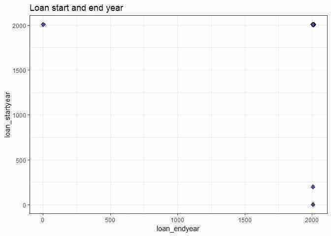
Scatterplot showing loan start and end year.
Figure 9.3 Scatterplot showing loan start and end year.
We can see that there are three observations that have very low (< 500) start or end year values, which does not make sense. We will replace these with ‘NA’, but leave the original data untouched and create a new dataset called
gotLc, where the ‘c’ indicates cleaned data.gotLc gotL gotLc$loan_startyear[gotLc$loan_startyear < 500] NA gotLc$loan_endyear[gotLc$loan_endyear < 500] NA ggplot(gotLc, aes(x = loan_endyear, y = loan_startyear)) + geom_point(size = 2, shape = 23, fill = "blue") + theme_bw() + ggtitle("Loan start and end year")In the top left corner, there is a loan with the start year (2006) after the end year (2003). Clearly this is incorrect, so we should remove this observation when analysing loan periods. However, we wait until we have combined the years with the months as there may be more observations with this issue.
Also, we can only see a small number of points because there are many identical observations (for example
startyearof 2006 andendyearof 2006). To see these points you could replacegeom_pointwithgeom_jitterin the command aboveggplotcommand . Use?geom_jitterto understand what this option does.Now let’s look at the values in
start_month.summary(gotLc$loan_startmonth)## April August December February January July June ## 95 63 133 145 176 115 156 ## March May November October September NA's ## 85 141 115 106 146 4There is no particular issue with the start months. What about the end months?
summary(gotLc$loan_endmonth)## April August December February January July June ## 136 53 49 170 52 34 94 ## March May November October Pagume September NA's ## 155 89 33 39 5 37 534Two things are noteworthy here: there are now many ‘NA’ entries, and there is an entry called ‘Pagume’. As described in the task, ‘Pagume’ can be approximated by September. Let’s recode that.
gotLc$loan_endmonth[gotLc$loan_endmonth == "Pagume"]
  "September"
Another call of
summary(gotLc$loan_endmonth)would confirm that there are no observations with ‘Pagume’ left.Now we want to calculate the length of the loan, in other words, the number of days between start and end day. As we only have months and not days, this will be an approximation. We will create a new variable combining months and years using the
pastefunction, assuming that all loan start and end dates are on the first day of each month.# We assume that all loan start and end dates are on the # 1st of the month. gotLc$loan_startdate paste("1", gotLc$loan_startmonth, gotLc$loan_startyear) gotLc$loan_enddate paste("1", gotLc$loan_endmonth, gotLc$loan_endyear)For observations with an unknown end date (recall we had more than 500 of these), we will code as missing. Currently these are recorded as ‘1 NA NA’. First we need to find which observations have missing data elements for either the
loan_startdateorloan_enddatevariable. R has very powerful tools to identify text patterns such as this, which you can learn about by searching the Internet for help (you could search for ‘R test whether character contains string’). For example, a useful short introduction to using such tools contains one solution to our problem.See the first 20 observations of
loan_enddate.gotLc$loan_enddate[1:20]## [1] "1 NA NA" "1 NA NA" "1 June 2006" ## [4] "1 March 2006" "1 February 2006" "1 September 2007" ## [7] "1 March 2006" "1 March 2006" "1 March 2006" ## [10] "1 March 2006" "1 February 2006" "1 NA NA" ## [13] "1 August 2007" "1 August 2007" "1 February 2006" ## [16] "1 June 2007" "1 November 2007" "1 March 2006" ## [19] "1 April 2006" "1 NA NA"You can find NAs in observations 1, 2, 12, and 20. The command
grepwill identify these rows automatically.# Identify the position of the observations that contain # NAs selNA grep('NA', gotLc$loan_enddate) selNA[1:5]## [1] 1 2 12 20 26As you can see,
grepidentifies the first four instances correctly, and we can see that the next missing end date is in observation 26. Now we will replace all these observations as missing values and then convert the non-missing observations to dates, using theas.Datefunction.gotLc$loan_enddate[selNA] NA gotLc$loan_enddate as.Date(gotLc$loan_enddate, format = "%d %B %Y")The option
format = "%d %B %Y"specifies the format that dates are recorded as (for example ‘1 June 2006’), where%Bstands for full months (view this page for examples of other date formatting options). Now we repeat the same steps for the start date.# Identify the position of the observations that contain # NAs selNA grep('NA', gotLc$loan_startdate) gotLc$loan_startdate[selNA] NA gotLc$loan_startdate as.Date(gotLc$loan_startdate, format = "%d %B %Y")Let’s use the
is.nafunction to find out the percentage of observations with missing values for start and/or end date. Here, we used thepastefunction to print the output as both a number and a percentage.# Missing start dates paste(sum(is.na(gotLc$loan_startdate)), "(", 100 * round(mean(is.na(gotLc$loan_startdate)), 4), "% )")## [1] "6 ( 0.41 % )"# Missing end dates paste(sum(is.na(gotLc$loan_enddate)), "(", 100 * round(mean(is.na(gotLc$loan_enddate)), 4), "% )")## [1] "535 ( 36.15 % )"Now we will add a new variable indicating the length of the loan period. As R knows that
loan_startdateandloan_enddateare dates, it recognizes automatically that the difference between two dates should be expressed as the number of days.gotLc$loan_length gotLc$loan_enddate-gotLc$loan_startdateLet’s look at the first few observations.
gotLc[1:5, c("loan_startdate",
 "loan_enddate", "loan_length")]
## # A tibble: 5 x 3 ## loan_startdate loan_enddate loan_length #### 1 2004-03-01 NA ## 2 2006-11-01 NA ## 3 2006-11-01 2006-06-01 -153 ## 4 2005-06-01 2006-03-01 273 ## 5 2005-06-01 2006-02-01 245 Notice the following:
- Where any of the two dates is missing, the length is missing as well.
- Some loan lengths are negative (for example observation 3), because the recorded end date is before the start date. It could be that the two dates were switched when the data was entered into the system.
This is unfortunate, but is a common feature of real-life data, and you will have to be on the lookout for such occasions.
As required in Question 1, we will create two variants of the
loan_lengthvariable: one where we assign missing values to all observations that have negativeloan_length, and one where we assume that the problem was the switching of start and end date, so we transform all loan lengths to positive values.gotLc$loan_length_NA gotLc$loan_length # Assign NA to negative loan lengths gotLc$loan_length_NA[gotLc$loan_length_NA<0] NA gotLc$loan_length_abs abs(gotLc$loan_length)Now we can create the
long_termvariable and look at the number of long-term loans.gotLc$long_term (gotLc$loan_length_abs>365) summary(gotLc$long_term)## Mode FALSE TRUE NA's ## logical 728 215 537We therefore have about 23% long-term loans (only looking at loans for which we do have date information).
- Using the variables
loan_amountandloan_interest:
- Create summary tables to summarize the distribution of loan amount (mean, standard deviation, maximum, and minimum): one using the loan amount, the other using the total amount to repay (loan amount + interest). Make sure to exclude the one observation previously identified as having an extremely high interest rate. Remember to give your tables meaningful titles. Describe any features of the data that you find interesting.
- As mentioned earlier, the interest rate is a borrowing condition that can vary widely across households. Here we will take the interest rate to be the interest paid as a percentage of the loan amount. Calculate the interest rate for each loan in the data. (Exclude observations where the interest paid is not recorded.)
- Check for extreme values (interest rates that are either very large or zero). You may also want to create a scatterplot (with interest rate on the vertical axis and loan amount on the horizontal axis) to help you identify extreme (atypical) observations. Exclude the observation with the most extreme interest rate from further calculations. What percentage of the loans are zero interest?
- Make summary tables of the mean, maximum, minimum, and quartiles of the loan amount and interest rate, calculating these measures separately for long-term and short-term loans. Compare the distributions of interest rates for short-term and long-term loans.
- Create a table showing the correlation between the interest rate and household characteristics (you may want to refer to Figure 8.4 in Empirical Project 8 for an example). Interpreting the interest rate charged as a measure of default risk (inability to repay), explain whether the relationships implied by the coefficients are what you expected (for example, would you expect interest rates to be higher for households with less assets, more dependents, etc.).
R walk-through 9.10 Making summary tables and calculating correlations
To make summary tables, we use the
favstatsfunction from themosaicpackage.# loan_amount favstats(~loan_amount, data = gotLc)## min Q1 median Q3 max mean sd n missing ## 1 400 1200 3490 3e+07 26896 783587 1479 1# loan_amount + loan_interest favstats(~(loan_amount + loan_interest), data = gotLc)## min Q1 median Q3 max mean sd n missing ## 20 500 1400 3780 31260000 29223 827144 1445 35It is best to look at loan amounts and interest rate graphically, for example in a scatterplot.
ggplot(gotLc, aes(x = loan_amount, y = loan_interest)) + geom_point(size = 2, shape = 23, fill = "blue") + theme_bw() + ggtitle("Loan amounts and interest payments")One large loan (top right corner) dominates this graph. Let’s exclude observations with a loan amount larger than 200,000 from the graph.
ggplot(gotLc, aes(x = loan_amount, y = loan_interest)) + geom_point(size = 2, shape = 23, fill = "blue") + # Set horizontal axis limits xlim(0, 200000) + # Set vertical axis limits ylim(0, 30000) + theme_bw() + ggtitle("Loan amounts and interest payments")Interestingly we can see many zero interest loans. Now we will calculate the interest rate as
loan_interest/loan_amount.gotLc$interest_rate gotLc$loan_interest / gotLc$loan_amount favstats(~interest_rate, data = gotLc)## min Q1 median Q3 max mean sd n missing ## 0 0 0 0.167 200 0.257 5.26 1445 35The maximum interest rate is 200 (in other words 20,000%), which does not make sense and could be due to a data entry error. Making another scatterplot can also identify extreme values for loan amounts.
ggplot(gotLc, aes(x = loan_amount, y = interest_rate)) +
  geom_point(size = 2, shape = 23, fill = "blue") +
  theme_bw() +
  ggtitle("Loan amounts and interest rates")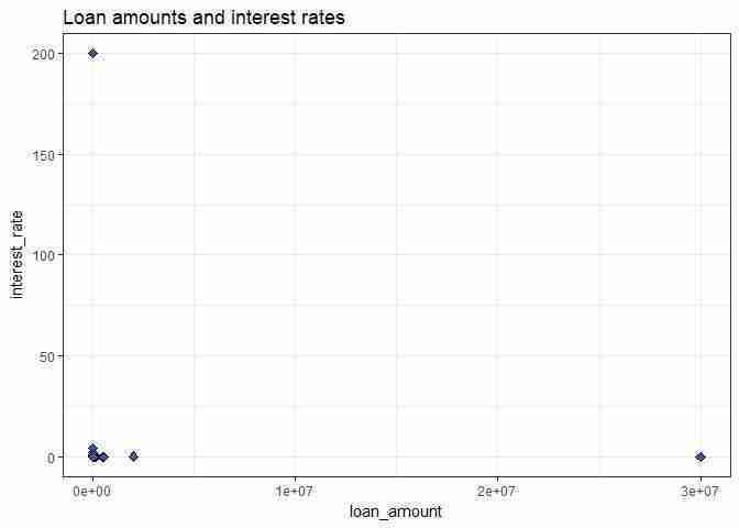
Scatterplot identifying extreme values for loan amounts.
Figure 9.7 Scatterplot identifying extreme values for loan amounts.
Let’s make another scatterplot, excluding the observation with the extremely high interest rate and only looking at small loan amounts (
ggplot(subset(gotLc, interest_rate < 50), aes(x = loan_amount, y = interest_rate)) + geom_point(size = 2, shape = 23, fill = "blue") + # Set horizontal axis limits xlim(0, 1000) + # Set vertical axis limits ylim(0, 5) + theme_bw() + ggtitle("Loan amount and interest rates")Again we can see that there are many zero interest loans. From the summary statistics above, we can see that the median interest rate is 0, which implies that at least 50% of loans have a zero interest rate. The following code calculates that percentage precisely.
temp_all  gotLc$interest_rate[
  !is.na(gotLc$interest_rate)]

temp_0  temp_all[temp_all == 0]

paste("Percentage of zero interest rate loans: ",
  round(100 * length(temp_0) / length(temp_all), 2),
  "%")
## [1] "Percentage of zero interest rate loans: 50.52 %"Now let’s calculate statistics conditional on whether a loan is long term or not. Before we do this, we will remove the observation with the very extreme interest rate (20,000%) from our ‘gotLc’ dataset (but not from the original ‘gotL’ dataset). That observation has a loan amount of 1 and an interest payment of 200, which is probably a data entry mistake. There is another extreme observation (with a loan amount of 30,000,000), but there is no indication that this observation is misrecorded as there is a significant interest payment for this loan.
gotLc  subset(gotLc, interest_rate < 200)

favstats(~interest_rate | long_term, data = gotLc)
## long_term min Q1 median Q3 max mean sd n missing ## 1 FALSE 0 0 0.050 0.171 1.12 0.110 0.173 717 0 ## 2 TRUE 0 0 0.141 0.245 2.24 0.189 0.268 211 0Both the mean and median interest rate are higher for long-term loans. You can adapt the code above to calculate statistics for the
loan_amountvariable.We now calculate correlations between interest rates and household characteristics. Below we use piping operations (
%>%) to select the relevant data (as in Project 8). We store the correlation coefficients in a matrix (array of rows and columns) calledM.gotLc %>% # Only select observations with interest rate information subset(!is.na(interest_rate)) %>% select(age, max_education, number_assets, hhsize, young_children, working_age_adults, interest_rate) %>% cor(., use = "pairwise.complete.obs") -> M M[, c("interest_rate")]## age max_education number_assets ## 0.0258 -0.0841 -0.0474 ## hhsize young_children working_age_adults ## 0.1050 0.1022 0.0466 ## interest_rate ## 1.0000
- Now we will look at sources of finance and how they are related to loan characteristics.
- Create a table showing the proportion of loans (in terms of the column variable) with source of finance (
borrowed_from) as the row variable andruralas the column variable. Make a similar table but withborrowed_from_otheras the row variable instead. Does it look like rural households use different sources of finance from urban households? (Hint: It may help to think about sources of finance in terms of formal, informal, and other institutions such as microfinancers or NGOs.)
-
For each of the variables below, create a table showing the average of that variable, with
borrowed_fromas the row variable andruralas the column variable. Comment on any similarities or differences between rows and columns that you find interesting, and suggest explanations for what you observe.- duration of loan (using the variable in which negative durations were transformed to positive durations)
- loan amount
- interest rate
- Create a table showing the proportion of
gender(in terms of the row variable) withborrowed_fromas the row variable andruralas the column variable. Describe any relationships you observe between the gender of household head, the place where he/she lives, and the types of finance used.
- What other variables are currently not in our dataset but could also be important for our analysis in Questions 2 and 3?
R walk-through 9.11 Creating summary tables of means
First we use the
tablefunction to create the table with the variableborrowed_from.stab10 table(gotLc$borrowed_from, gotLc$rural) addmargins(prop.table(stab10, 2), 1)## ## Large town (urban) Rural Small town (urban) ## Bank (commercial) 0.01881 0.00393 0.00000 ## Employer 0.04075 0.00196 0.01031 ## Grocery/Local Merchant 0.08150 0.04711 0.10309 ## Microfinance Institution 0.19122 0.27969 0.26804 ## Money Lender (Katapila) 0.00313 0.04809 0.02062 ## NGO 0.01254 0.04711 0.05155 ## Neighbour 0.10658 0.11580 0.07216 ## Other (specify) 0.05643 0.12071 0.04124 ## Relative 0.48589 0.31501 0.43299 ## Religious Institution 0.00313 0.02061 0.00000 ## Sum 1.00000 1.00000 1.00000Note that in all settings, most loans come from relatives. To create the table with
borrowed_from_other, substitute this variable name in the above command.When creating a table with categorical (factor) variables in the rows and columns, but with the cells reporting a statistic based on a third variable such as the average duration of a loan (rather than counts or proportions), we use piping operations (
%>%).tab10 gotLc %>% group_by(borrowed_from, rural) %>% summarize(mean_duration = round(mean(loan_length_abs, na.rm = TRUE), 0)) %>% spread(rural, mean_duration) %>% print()## # A tibble: 11 x 4 ## # Groups: borrowed_from [11] ## borrowed_from `Large town (urban)` Rural `Small town (urba~ #### 1 Bank (commercial) 1814 619 ## 2 Employer 602 290 NaN ## 3 Grocery/Local Merchant 166 259 176 ## 4 Microfinance Institution 712 411 510 ## 5 Money Lender (Katapila) 365 332 365 ## 6 Neighbour 125 187 296 ## 7 NGO 372 395 236 ## 8 Other (specify) 274 372 806 ## 9 Relative 237 217 393 ## 10 Religious Institution 1461 343 ## 11 1096 289 151 To get the tables for the loan amount and interest rate, change the variable name in the
mean()calculation above.Extension
Investigating sources of finance associated with zero interest loans
We previously saw that a large percentage of loans have a zero interest rate. Here we investigate whether particular sources of finance are responsible for these interest rates. The code we use is very similar to the code above, but instead of calculating the mean of a variable, we calculate the mean of a boolean (true/false) variable (
(interest_rate==0)). This will deliver the proportion of ‘true’ observations, in other words, loans where the interest rate was equal to zero.tab10 gotLc %>% group_by(borrowed_from, rural) %>% summarize(prop_0_interest = mean((interest_rate == 0), na.rm = TRUE)) %>% spread(rural, prop_0_interest) %>% print()## # A tibble: 11 x 4 ## # Groups: borrowed_from [11] ## borrowed_from `Large town (urban)` Rural `Small town (urba~ #### 1 Bank (commercial) 0. 0. NA ## 2 Employer 0.692 0.500 1.00 ## 3 Grocery/Local Merchant 1.00 0.812 1.00 ## 4 Microfinance Institution 0.0820 0.0351 0.0385 ## 5 Money Lender (Katapila) 0. 0.0204 0.500 ## 6 NGO 0.250 0.0833 0.400 ## 7 Neighbour 1.00 0.763 1.00 ## 8 Other (specify) 0.222 0.171 0. ## 9 Relative 0.961 0.819 0.976 ## 10 Religious Institution 1.00 0.190 NA ## 11 0. 0.571 1.00 You can see that in both urban and rural settings, a high proportion of loans granted by local merchants, neighbours, and relatives are zero interest (possibly because these people have a close relationship with the borrower so there is a lower chance of default).
We will use exactly the same technique to determine the proportion of loans that go to households with female heads.
tab11  gotLc %>%
  group_by(borrowed_from, rural) %>%
  summarize(prop_female = mean((gender == "Female"),
    na.rm = TRUE)) %>%
  spread(rural, prop_female) %>%
  print()
## # A tibble: 11 x 4 ## # Groups: borrowed_from [11] ## borrowed_from `Large town (urban)` Rural `Small town (urban~ #### 1 Bank (commercial) 0. 0.500 NA ## 2 Employer 0.308 0. 0. ## 3 Grocery/Local Merchant 0.385 0.188 0.500 ## 4 Microfinance Institution 0.410 0.130 0.308 ## 5 Money Lender (Katapila) 0. 0.265 0.500 ## 6 NGO 0.250 0.312 0.200 ## 7 Neighbour 0.353 0.254 0.429 ## 8 Other (specify) 0.389 0.187 0.250 ## 9 Relative 0.400 0.206 0.286 ## 10 Religious Institution 1.00 0.238 NA ## 11 1.00 0.429 1.00
- In this project we have looked at patterns in borrowing and access to credit, but we are not able to make any causal statements such as ‘changes in X will cause households to be credit constrained’ or ‘characteristic Y causes improved access to credit’. Outline a policy intervention that could help improve households’ access to loans, and how to design the implementation so you can assess the causal effects of this policy.
