Empirical Project 5 Working in R

Download the code

To download the code chunks used in this project, right-click on the download link and select ‘Save Link As…’. You’ll need to save the code download to your working directory, and open it in RStudio.

Don’t forget to also download the data into your working directory by following the steps in this project.

R-specific learning objectives

In addition to the learning objectives for this project, in Part 5.1 you will learn how to use loops to repeat specified tasks for a list of values (Note: this is an extension task so may not apply to all users).

Getting started in R

For this project you will need the following packages:

tidyverse, to help with data manipulation
readxl, to import an Excel spreadsheet
ineq, to calculate inequality measures
reshape2, to rearrange a dataframe.

If you need to install any of these packages, run the following code:

install.packages(c(
  "readxl", "tidyverse",
  "ineq", "reshape2"))

You can import these libraries now, or when they are used in the R walk-throughs below.

library(readxl)
library(tidyverse)
library(ineq)
library(reshape2)

Part 5.1 Measuring income inequality

Learning objectives for this part

draw Lorenz curves

calculate and interpret the Gini coefficient

interpret alternative measures of income inequality.

One way to visualize the income distribution in a population is to draw a Lorenz curve. This curve shows the entire population lined up along the horizontal axis from the poorest to the richest. The height of the curve at any point on the vertical axis indicates the fraction of total income received by the fraction of the population given by that point on the horizontal axis.

We will start by using income decile data from the Global Consumption and Income Project to draw Lorenz curves and compare changes in the income distribution of a country over time. Note that income here refers to market income, which does not take into account taxes or government transfers (see Section 5.10 of Economy, Society, and Public Policy for further details).

To answer the question below:

Go to the Globalinc website and download the Excel file containing the data by clicking ‘xlsx’.
Save it in an easily accessible location, such as a folder on your Desktop or in your personal folder.
Import the data into R as explained in R walk-through 5.1.

R walk-through 5.1 Importing an Excel file (either .xlsx or .xls format) into R

As we are importing an Excel file, we use the read_excel function from the readxl package. The file is called GCIPrawdata.xlsx. Before you import the file into R, open the datafile in Excel to understand its structure. You will see that the data is all in one worksheet (which is convenient), and that the headings for the variables are in the third row. Hence we will use the skip = 2 option in the read_excel function to skip the first two rows.
library(tidyverse)  
library(readxl) 

# Set your working directory to the correct folder.
# Insert your file path for 'YOURFILEPATH'.
setwd("YOURFILEPATH")

decile_data  read_excel("GCIPrawdata.xlsx", skip = 2)  
The data is now in a ‘tibble’ (like a spreadsheet for R). Let’s use the head function to look at the first few rows:
head(decile_data)  
## # A tibble: 6 x 14
##   Country      Year `Decile 1 Income` `Decile 2 Income` `Decile 3 Income`
##                                                 
## 1 Afghanistan  1980               206               350               455
## 2 Afghanistan  1981               212               361               469
## 3 Afghanistan  1982               221               377               490
## 4 Afghanistan  1983               238               405               527
## 5 Afghanistan  1984               249               424               551
## 6 Afghanistan  1985               256               435               566
## # ... with 9 more variables: `Decile 4 Income` , `Decile 5
## #   Income` , `Decile 6 Income` , `Decile 7 Income` ,
## #   `Decile 8 Income` , `Decile 9 Income` , `Decile 10
## #   Income` , `Mean Income` , Population 
As you can see, each row shows data for a different country-year combination. The first row is for Afghanistan in 1980, and the first value (in the third column) is 206, for the variable Decile 1 Income. This value indicates that the mean annual income of the poorest 10% in Afghanistan was the equivalent of 206 USD (in 1980, adjusted using purchasing power parity). Looking at the next column, you can see that the mean income of the next richest 10% (those in the 11th to 20th percentiles for income) was 350.

To see the list of variables, we use the str function.
str(decile_data)  
## Classes 'tbl_df', 'tbl' and 'data.frame':  4799 obs. of 14 variables:
##  $ Country         : chr  "Afghanistan" "Afghanistan" "Afghanistan" "Afghanistan" ...
##  $ Year            : num  1980 1981 1982 1983 1984 ...
##  $ Decile 1 Income : num  206 212 221 238 249 256 268 243 223 202 ...
##  $ Decile 2 Income : num  350 361 377 405 424 435 457 414 380 344 ...
##  $ Decile 3 Income : num  455 469 490 527 551 566 594 539 493 447 ...
##  $ Decile 4 Income : num  556 574 599 644 674 692 726 659 603 547 ...
##  $ Decile 5 Income : num  665 686 716 771 806 828 869 788 722 654 ...
##  $ Decile 6 Income : num  793 818 854 919 961 ...
##  $ Decile 7 Income : num  955 986 1029 1107 1157 ...
##  $ Decile 8 Income : num  1187 1225 1278 1376 1438 ...
##  $ Decile 9 Income : num  1594 1645 1717 1848 1932 ...
##  $ Decile 10 Income: num  3542 3655 3814 4105 4291 ...
##  $ Mean Income     : num  1030 1063 1109 1194 1248 ...
##  $ Population      : num  13211412 12996923 12667001 12279095 11912510 ...
In addition to the country, year, and the ten income deciles, we have mean income and the population.

To draw Lorenz curves, we need to calculate the cumulative share of total income owned by each decile (these will be the vertical axis values). The cumulative income share of a particular decile is the proportion of total income held by that decile and all the deciles below it. For example, if Decile 1 has 1/10 of total income and Decile 2 has 2/10 of total income, the cumulative income share of Decile 2 is 3/10 (or 0.3).

Choose two countries. You will be using their data, for 1980 and 2014, as the basis for your Lorenz curves. Use the country data you have selected to calculate the cumulative income share of each decile. (Remember that each decile represents 10% of the population.)

R walk-through 5.2 Calculating cumulative shares using the `cumsum` function

Here we have chosen China (a country that recently underwent enormous economic changes) and the US (a developed country). We use the subset function to create a new dataset (called temp) containing only the countries and years we need.

#  Select the data for the chosen country and years
sel_Year  c(1980, 2014)
sel_Country  c("United States", "China")

temp  subset(
  decile_data, 
  (decile_data$Country %in% sel_Country) & 
  (decile_data$Year %in% sel_Year))
temp

## # A tibble: 4 x 14
##   Country        Year `Decile 1 Income` `Decile 2 Income` `Decile 3 Incom~
##                                                  
## 1 China          1980                79               113              146
## 2 China          2014               448               927             1440
## 3 United States  1980              3392              5820             7855
## 4 United States  2014              3778              6534             9069
## # ... with 9 more variables: `Decile 4 Income` , `Decile 5
## #   Income` , `Decile 6 Income` , `Decile 7 Income` ,
## #   `Decile 8 Income` , `Decile 9 Income` , `Decile 10
## #   Income` , `Mean Income` , Population 

Before we calculate cumulative income shares, we need to calculate the total income for each country-year combination using the mean income and the population size.

print("Total incomes are:")  

## [1] "Total incomes are:"

total_income  temp[, "Mean Income"] * 
  temp[, "Population"]  
total_income  

##   Mean Income  
## 1 2.472624e+11  
## 2 6.609944e+12  
## 3 3.366422e+12  
## 4 6.401280e+12  

These numbers are very large, so for our purpose it is easier to assume that there is only one person in each decile, in other words the total income is 10 times the mean income. This simplification works because, by definition, each decile has exactly the same number of people (10% of the population).

We will be using the very useful cumsum function (short for ‘cumulative sum’) to calculate the cumulative income. To see what this function does, look at this simple example.

test  c(2, 4, 10, 22)  
cumsum(test)  

## [1] 2 6 16 38

You can see that each number in the sequence is the sum of all the preceding numbers (including itself), for example, we got the third number, 16, by adding 2, 4, and 10. We now apply this function to calculate the cumulative income shares for China (1980) and save them as cum_inc_share_c80.

# Pick the deciles (Columns 3 to 12) in Row 1 (China, 1980)
decs_c80  unlist(temp[1, 3:12])
                               
# The unlist function transforms temp[1, 3:12] from a 
# tibble to simple vector with data which simplifies the 
# calculations.

# Give the total income, assuming a population of 10
total_inc  10 * unlist(temp[1, "Mean Income"])

cum_inc_share_c80 = cumsum(decs_c80) / total_inc
cum_inc_share_c80

##  Decile 1 Income  Decile 2 Income  Decile 3 Income  Decile 4 Income 
##       0.03134921       0.07619048       0.13412698       0.20436508 
##  Decile 5 Income  Decile 6 Income  Decile 7 Income  Decile 8 Income 
##       0.28769841       0.38492063       0.49841270       0.63174603 
##  Decile 9 Income Decile 10 Income 
##       0.79206349       0.99841270

We repeat the same process for China in 2014 (cum_inc_share_c14) and for the US in 1980 and 2014 (cum_inc_share_us80 and cum_inc_share_us14 respectively).

# For China, 2014  
# Go to Row 2 (China, 2014)
decs_c14  unlist(temp[2, 3:12])

# Give the total income, assuming a population of 10
total_inc  10 * unlist(temp[2, "Mean Income"]) 

cum_inc_share_c14 = cumsum(decs_c14) / total_inc  
  
# For the US, 1980  
# Select Row 3 (USA, 1980)
decs_us80  unlist(temp[3, 3:12])

# Give the total income, assuming a population of 10
total_inc  10 * unlist(temp[3, "Mean Income"])

cum_inc_share_us80 = cumsum(decs_us80) / total_inc  
  
# For the US, 2014  
# Select Row 4 (USA, 2014)
decs_us14  unlist(temp[4, 3:12])   

# Give the total income, assuming a population of 10 
total_inc  10 * unlist(temp[4, "Mean Income"])

cum_inc_share_us14 = cumsum(decs_us14) / total_inc  

Use the cumulative income shares to draw Lorenz curves for each country in order to visually compare the income distributions over time.

Draw a line chart with cumulative share of population on the horizontal axis and cumulative share of income on the vertical axis. Make sure to include a chart legend, and label your axes and chart appropriately.

Follow the steps in R walk-through 5.3 to add a straight line representing perfect equality to each chart. (Hint: If income was shared equally across the population, the bottom 10% of people would have 10% of the total income, the bottom 20% would have 20% of the total income, and so on.)

R walk-through 5.3 Drawing Lorenz curves

Let us plot the cumulative income shares for China (1980), which we previously stored in the variable cum_inc_share_c80. The plot function makes the basic chart, with the cumulative income share in blue. We then use the functions abline to add the perfect equality line (in black), and title to add a chart title.
plot(cum_inc_share_c80, type = "l", col = "blue", 
  lwd = 2, ylab = "Cumulative income share")  

# Add the perfect equality line 
abline(a = 0, b = 0.1, col = "black", lwd = 2)

title("Lorenz curve, China, 1980") 
Lorenz curve, China, 1980.

Figure 5.1 Lorenz curve, China, 1980.

The blue line is the Lorenz curve. The Gini coefficient is the ratio of the area between the two lines and the total area under the black line. We will calculate the Gini coefficient in R walk-through 5.4.

Now we add the other Lorenz curves to the chart using the lines function. We use the col= option to specify a different colour for each line, and the lty option to make the line pattern solid for 2014 data and dashed for 1980 data. Finally, we use the legend function to add a chart legend in the top left corner of the chart.
plot(cum_inc_share_c80, type = "l", col = "blue", 
  lty = 2, lwd = 2, xlab = "Deciles", 
  ylab = "Cumulative income share")  

# Add the perfect equality line 
abline(a = 0, b = 0.1, col = "black", lwd = 2)  

# lty = 1 = dashed line  
lines(cum_inc_share_c14, col = "green", lty = 1, lwd = 2)

# lty = 2 = solid line  
lines(cum_inc_share_us80, col = "red", lty = 2, lwd = 2)

lines(cum_inc_share_us14, col = "orange", 
  lty = 1, lwd = 2)  

title("Lorenz curves, China and the US (1980 and 2014)")  

legend("topleft", lty = 2:1, lwd = 2, cex = 1.2, legend = 
  c("China, 1980", "China, 2014",
    "US, 1980", "US, 2014"),  
  col = c("blue", "green", "red", "orange"))  
Lorenz curves, China and the US (1980 and 2014).

Figure 5.2 Lorenz curves, China and the US (1980 and 2014).

As the chart shows, the income distribution has changed more clearly for China (from the blue to the green line) than for the US (from the orange to the red line).

Using your Lorenz curves:

Compare the distribution of income across time for each country.

Compare the distribution of income across countries for each year (1980 and 2014).

Suggest some explanations for any similarities and differences you observe. (You may want to research your chosen countries to see if there were any changes in government policy, political events, or other factors that may affect the income distribution.)

A rough way to compare income distributions is to use a summary measure such as the Gini coefficient. The Gini coefficient ranges from 0 (complete equality) to 1 (complete inequality). It is calculated by dividing the area between the Lorenz curve and the perfect equality line, by the total area underneath the perfect equality line. Intuitively, the further away the Lorenz curve is from the perfect equality line, the more unequal the income distribution is, and the higher the Gini coefficient will be.

To calculate the Gini coefficient you can either use a Gini coefficient calculator, or calculate it directly in R as shown in R walk-through 5.4.

Calculate the Gini coefficient for each of your Lorenz curves. You should have four coefficients in total. Label each Lorenz curve with its corresponding Gini coefficient, and check that the coefficients are consistent with what you see in your charts.

R walk-through 5.4 Calculating Gini coefficients

The Gini coefficient is graphically represented by dividing the area between the perfect equality line and the Lorenz curve by the total area under the perfect equality line (see Section 5.9 of Economy, Society, and Public Policy for further details). You could calculate this area manually, by decomposing the area under the Lorenz curve into rectangles and triangles, but as with so many problems, someone else has already figured out how to do that and has provided R users with a package (called ineq) that does this task for you. The function that calculates Gini coefficients from a vector of numbers is called Gini, and we apply it to the income deciles from R walk-through 5.3 (decs_c80, decs_c14, decs_us80, and decs_us14).
# Load the ineq library
library(ineq)

# The decile mean incomes from R walk-through 5.3 are used.
g_c80  Gini(decs_c80)
g_c14  Gini(decs_c14)
g_us80  Gini(decs_us80)
g_us14  Gini(decs_us14)
paste("Gini coefficients")
## [1] "Gini coefficients"
paste("China - 1980: ", round(g_c80, 2), 
  ", 2014: ", round(g_c14, 2))
## [1] "China - 1980: 0.29 , 2014: 0.51"
paste("United States - 1980: ", round(g_us80, 2), 
  ", 2014: ", round(g_us14, 2))
## [1] "United States - 1980: 0.34 , 2014: 0.4"
Now we make the same line chart (simply copy and paste the code from R walk-through 5.3, but use the text function to label curves with their respective Gini coefficients. The two numbers in the text function specify the coordinates (horizontal and vertical) where the text should be written (experiment for yourself to find the best place to put the labels), and we used the round function to show the first three digits of the calculated Gini coefficients.
plot(cum_inc_share_c80, type = "l", col = "blue", lty = 2, 
  lwd = 2, xlab = "Deciles", 
  ylab = "Cumulative income share")   

# Add the perfect equality line
abline(a = 0, b = 0.1, col = "black", lwd = 2)

# lty = 1 = dashed line
lines(cum_inc_share_c14, col = "green", lty = 1, lwd = 2)

# lty = 2 = solid line
lines(cum_inc_share_us80, col = "red", lty = 2, lwd = 2)

lines(cum_inc_share_us14, col = "orange", lty = 1, lwd = 2)

title("Lorenz curves, China and the US (1980 and 2014)")

legend("topleft", lty = 2:1, lwd = 2, cex = 1.2, legend = 
  c("China, 1980", "China, 2014", 
    "US, 1980", "US, 2014"),
  col = c("blue", "green", "red", "orange"))

text(8.5, 0.78, round(g_c80, digits = 3))
text(9.4, 0.6, round(g_c14, digits = 3))
text(5.7, 0.38, round(g_us80, digits = 3))
text(6.4, 0.3, round(g_us14, digits = 3))
Lorenz curves, China and the US (1980 and 2014).

Figure 5.3 Lorenz curves, China and the US (1980 and 2014).

The Gini coefficients for both countries have increased, confirming what we already saw from the Lorenz curves that in both countries the income distribution has become more unequal.

Extension R walk-through 5.5 Calculating Gini coefficients for all countries and all years using a loop

In this extension walk-through, we show you how to calculate the Gini coefficient for all countries and years in your dataset.

This sounds like a tedious task, and indeed if we were to use the same method as before it would be mind-numbing. However, we have a powerful programming language at hand, and this is the time to use it.

Here we use a very useful programming tool you may not have come across yet: loops. Loops are used to repeat a specified block of code. There are a few types of loop, and here we will use a ‘for’ loop, meaning that we ask R to apply the same code to each number or item in a specific list (i.e. repeat the code ‘for’ a list of numbers/items). Let’s start with a very simple case: printing the first 10 square numbers. In coding terms, we are printing the values for i^2 for the numbers i=1, ..., 10.
for (i in seq(1, 10)){
  print(i^2)
}
## [1] 1
## [1] 4
## [1] 9
## [1] 16
## [1] 25
## [1] 36
## [1] 49
## [1] 64
## [1] 81
## [1] 100
In the above command, seq(1, 10) creates a vector of numbers from 1 to 10 (1, 2, 3, …, 10). The command for (i in seq(1, 10)) defines the variable i initially as 1, then performs all the commands that are between the curly brackets for each value of i (typically these commands will involve the variable i). Here our command prints the value of i^2 for each value of i. Check that you understand the syntax above by modifying it to print only the first 5 square numbers, or adding 2 to the numbers from 1 to 10 (instead of squaring these numbers).

Now we use loops to complete our task. We begin by creating a new variable in our dataset, gini, which we initially set to 0 for all country-year combinations.
decile_data$gini  0
Now we use a loop to run through all the rows in our dataset (country-year combinations). For each row we will repeat the Gini coefficient calculation from R walk-through 5.4 and save the resulting value in the gini variable we created.
# Give us the number of rows in decile_data
noc  nrow(decile_data)

for (i in seq(1, noc)){
  # Go to Row I to get the decile data
  decs_i  unlist(decile_data[i, 3:12])
  decile_data$gini[i]  Gini(decs_i)
}
With this code, we calculated 4,799 Gini coefficients without having to manually run the same command 4,799 times. We now look at some summary measures for the gini variable.
summary(decile_data$gini)
## Min.   1st Qu. Median Mean   3rd Qu. Max.
## 0.1791 0.3470  0.4814 0.4617 0.5700  0.7386
The average Gini coefficient is 0.46, the maximum is 0.74, and the minimum 0.18. Let’s look at these extreme cases.

First we will look at the extremely equal income distributions (those with a Gini coefficient smaller than 0.20):
temp  subset(
  decile_data, decile_data$gini < 0.20, 
  select = c("Country", "Year", "gini"))
temp
## # A tibble: 17 x 3
##    Country          Year  gini
##                
##  1 Bulgaria         1987 0.191
##  2 Czech Republic   1985 0.195
##  3 Czech Republic   1986 0.194
##  4 Czech Republic   1987 0.192
##  5 Czech Republic   1988 0.191
##  6 Czech Republic   1989 0.194
##  7 Czech Republic   1990 0.196
##  8 Czech Republic   1991 0.199
##  9 Slovak Republic  1985 0.195
## 10 Slovak Republic  1986 0.194
## 11 Slovak Republic  1987 0.193
## 12 Slovak Republic  1988 0.192
## 13 Slovak Republic  1989 0.193
## 14 Slovak Republic  1990 0.194
## 15 Slovak Republic  1991 0.195
## 16 Slovak Republic  1992 0.196
## 17 Slovak Republic  1993 0.179
These correspond to eastern European countries before the fall of communism.

Now the most unequal countries (those with a Gini coefficient larger than 0.73):
temp  subset(
  decile_data, decile_data$gini > 0.73, 
  select = c("Country", "Year", "gini"))
temp
## # A tibble: 27 x 3
##    Country       Year  gini
##             
##  1 Burkina Faso  1980 0.738
##  2 Burkina Faso  1981 0.738
##  3 Burkina Faso  1982 0.738
##  4 Burkina Faso  1983 0.738
##  5 Burkina Faso  1984 0.738
##  6 Burkina Faso  1985 0.738
##  7 Burkina Faso  1986 0.738
##  8 Burkina Faso  1987 0.738
##  9 Burkina Faso  1988 0.738
## 10 Burkina Faso  1989 0.739
## # ... with 17 more rows

Extension R walk-through 5.6 Plotting time series of Gini coefficients, using ggplot

In this extension walk-through, we show you how to make time series plots (time on the horizontal axis, the variable of interest on the vertical axis) with Gini coefficients for a list of countries of your choice.

There are many ways to plot data in R, one being the standard plotting function (plot) we used in previous walk-throughs. Another (and perhaps more beautiful) way is to use the ggplot function, which is part of the tidyverse package we loaded earlier. Our dataset is already in a format which the ggplot function can easily use (the ‘long’ format, where each row corresponds to a different country-year combination).

First we use the subset function to select a small list of countries and save their data as temp_data. As an example, we have chosen four anglophone countries: the UK, the US, Ireland, and Australia.
temp_data  subset(
  decile_data, Country %in% c("United Kingdom", 
    "United States", "Ireland", "Australia"))
Now we plot the data using ggplot.
ggplot(temp_data, 
  aes(x = Year, y = gini, color = Country)) +
  geom_line(size = 1) +
  theme_bw() +
  ylab("Gini") +
  # Add a title
  ggtitle("Gini coefficients for anglophone countries")
Time series plots of Gini coefficients for anglophone countries.

Figure 5.4 Time series plots of Gini coefficients for anglophone countries.

We asked the ggplot function to use the temp_data dataframe, with Year on the horizontal axis (x = ) and gini on the vertical axis (y = ). The color option indicates which variable we use to separate the data (use a different line for each unique item in Country). The first line of code sets up the chart, and the + geom_line(size = 1) then instructs R to draw lines. (See what happens if you replace + geom_line(size = 1) with + geom_point(size = 1).)

ggplot assumes that the different lines you want to show are identified through the different values in one variable (here, the Country variable). If your data is formatted differently, for example, if you have one variable for the Gini of each country (‘wide’ format), then in order to use ggplot you will first have to transform the dataset into ‘long’ format. Doing so is beyond the scope of this task, however you can find a worked example online, such as ‘R TSplots’.¹ Project 4 also explains how to transform data between ‘wide’ and ‘long’ formats.

The ggplot package is extremely powerful, and if you want to produce a variety of different charts, you may want to read more about that package, for example, see a Harvard R tutorial or an R statistics tutorial for great examples that include code.

Now we will look at other measures of income inequality and see how they can be used along with the Gini coefficient to summarize a country’s income distribution. Instead of summarizing the entire income distribution like the Gini coefficient does, we can take the ratio of incomes at two points in the distribution. For example, the 90/10 ratio takes the ratio of the top 10% of incomes (Decile 10) to the lowest 10% of incomes (Decile 1). A 90/10 ratio of 5 means that the richest 10% earns 5 times more than the poorest 10%. The higher the ratio, the higher the inequality between these two points in the distribution.

Look at the following ratios:
- 90/10 ratio = the ratio of Decile 10 income to Decile 1 income
- 90/50 ratio = the ratio of Decile 10 income to Decile 5 income (the median)
- 50/10 ratio = the ratio of Decile 5 income (the median) to Decile 1 income.

For each of these ratios, explain why policymakers might want to compare these two deciles in the income distribution.

What kinds of policies or events could affect these ratios?

We will now compare these summary measures (ratios and the Gini coefficient) for a larger group of countries, using OECD data. The OECD has annual data for different ratio measures of income inequality for 42 countries around the world, and has an interactive chart function that plots them for you.

Go to the OECD website to access the data. You will see a chart similar to Figure 5.5, showing data for 2015. The countries are ranked from smallest to largest Gini coefficient on the horizontal axis, and the vertical axis gives the Gini coefficient.

Compare summary measures of inequality for all available countries on the OECD website:

Plot the data for the ratio measures by changing the variable selected in the drop-down menu ‘Gini coefficient’. The three ratio measures we looked at previously are called ‘Interdecile P90/P10’, ‘Interdecile P90/P50’, and ‘Interdecile P50/P10’, respectively. (If you click the ‘Compare variables’ option, you can plot more than one variable (except the Gini coefficient) on the same chart.)

For each measure, give an intuitive explanation of how it is measured and what it tells us about income inequality. (For example: What do the larger and smaller values of this measure mean? Which parts of the income distribution does this measure use?)

Do countries that rank highly on the Gini coefficient also rank highly on the ratio measures, or do the rankings change depending on the measure used? Based on your answers, explain why it is important to look at more than one summary measure of a distribution.

OECD countries ranked according to their Gini coefficient (2015).

Figure 5.5 OECD countries ranked according to their Gini coefficient (2015).

The Gini coefficient and the ratios we have used are common measures of inequality, but there are other ways to measure income inequality.

Go to the Chartbook of Economic Inequality, which contains five measures of income inequality, including the Gini coefficient, for 25 countries around the world.

Choose two measures of income inequality that you find interesting (excluding the Gini coefficient). For each measure, give an intuitive explanation of how it is measured and what we can learn about income inequality from it. You may find the page on ‘Inequality measures’ helpful. (For example: What do larger or smaller values of this measure mean? Which parts of the income distribution does this measure use?)

On the Chartbook of Economic Inequality main page, charts of these measures are available for all countries shown in green on the map. For two countries of your choice, look at the charts and explain what these measures tell us about inequality in those countries.

Part 5.2 Measuring other kinds of inequality

Learning objectives for this part

research other dimensions of inequality and how they are measured.

There are many ways to measure income inequality, but income inequality is only one dimension of inequality within a country. To get a more complete picture of inequality within a country, we need to look at other areas in which there may be inequality in outcomes. We will explore two particular areas:

health inequality
gender inequality in education.

First, we will look at how researchers have measured inequality in health-related outcomes. Besides income, health is an important aspect of wellbeing, partly because it determines how long an individual will be alive to enjoy his or her income. If two people had the same annual income throughout their lives, but one person had a much shorter life than the other, we might say that the distribution of wellbeing is unequal, despite annual incomes being equal.

As with income, inequality in life expectancy can be measured using a Gini coefficient. In the study ‘Mortality inequality’, researcher Sam Peltzman (2009) estimated Gini coefficients for life expectancy based on the distribution of total years lived (life-years) across people born in a given year (birth cohort). If everybody born in a given year lived the same number of years, then the total years lived would be divided equally among these people (perfect equality). If a few people lived very long lives but everybody else lived very short lives, then there would be a high degree of inequality (Gini coefficient close to 1).

We will now look at mortality inequality Gini coefficients for 10 countries around the world. First, download the data:

Go to the ‘Health Inequality’ section of the Our World in Data website. In Section 1.1 (Mortality inequality), click the ‘Data’ button at the bottom of the chart shown.
Click the blue button that appears to download the data in csv format.

Import the data into R and investigate the structure of the data as explained in R walk-through 5.7.

R walk-through 5.7 Importing .csv files into R

Before importing, make sure the .csv file is saved in your working directory. After importing (using the read.csv function), use the str function to check that the data was imported correctly.
# Open the csv file from the working directory
health_in  read.csv("
  inequality-of-life-as-measured-by-mortality-gini-coefficient-1742-2002.csv")
str(health_in)
## 'data.frame':  320 obs. of 4 variables:
##  $ Entity    : Factor w/ 10 levels "Brazil","England and Wales",..: 1 1 1 1 1 1 1 1 1 1 ...
##  $ Code      : Factor w/ 10 levels "","BRA","DEU",..: 2 2 2 2 2 2 2 2 2 2 ...
##  $ Year      : int  1892 1897 1902 1907 1912 1917 1922 1927 1932 1937 ...
##  $ X.percent.: num  0.566 0.557 0.547 0.482 0.494 ...
The variable Entity is the country and the variable X.percent is the health Gini. Let’s change these variable names (to Country and Health, respectively) to clarify what they actually refer to, which will help when writing code (and if we go back to read this code at a later date).
# Country is the first variable.
names(health_in)[1]  "Country"
# Health Gini is the fourth variable.
names(health_in)[4]  "HGini"
There is another quirk in the data that you may not have noticed in this initial data inspection: All countries have a short code (Code), except for England and Wales (currently blank "" in the dataframe). As Code is a factor variable, we use the levels function to change the blanks to "ENW".
levels(health_in$Code)[levels(health_in$Code) == ""]  
  "ENW"
Tip

The way this code works may seem a little mysterious, and you may find it difficult to remember the code for this step. However, an Internet search for ‘R renaming one factor level’ (recall that Code is a factor variable) will show you many ways to achieve this (including the one shown above). Often you will find answers on stackoverflow.com, where experienced coders provide useful help.

Using the mortality inequality data:

Plot all the countries on the same line chart, with Gini coefficient on the vertical axis and year (1952–2002 only) on the horizontal axis. Make sure to include a legend showing country names, and label the axes appropriately.

Describe any general patterns in mortality inequality over time, as well as any similarities and differences between countries.

R walk-through 5.8 Creating line graphs with ggplot

As shown in R walk-through 5.7, the data is already formatted so that we can use ggplot directly (in ‘long’ format), in other words we have only one variable for the mortality Gini (HGini), and we can separate the data by country using one variable (Country).

Most of the code below is similar to our use of ggplot in previous walk-throughs, though this time we added the option labs to change the vertical axis label (y = ) and the option scale_color_brewer to change the colour palette (to clearly differentiate the lines for each country).
# Select all data after 1951
temp_data  subset(health_in, Year > 1951)

ggplot(temp_data, 
  aes(x = Year, y = HGini, color = Country)) +
  geom_line(size = 1) +
  labs(y = "Mortality inequality Gini coefficient") +
  # Change the colour palette
  scale_color_brewer(palette = "Paired") +
  theme_bw() +
  # Add a title
  ggtitle("Mortality inequalities")
Mortality inequality Gini coefficients (1952–2002).

Figure 5.6 Mortality inequality Gini coefficients (1952–2002).

Now compare the Gini coefficients in the first year of your line chart (1952) with the last year (2002).

For the year 1952, sort the countries according to their mortality inequality Gini coefficient from smallest to largest. Plot a column chart showing these Gini coefficients on the vertical axis, and country on the horizontal axis.

Repeat Question 2(a) for the year 2002.

Comparing your charts for 1952 and 2002, have the rankings between countries changed? Suggest some explanations for any observed changes. (You may want to do some additional research, for example, look at the healthcare systems of these countries.)

R walk-through 5.9 Drawing a column chart with sorted values

Plot a column chart for 1952

First we use subset to extract the data for 1952 only, and store it in a temporary dataset (tempdata).
# Select all data for 1952
temp_data  subset(health_in, Year == 1952)

# Reorder rows in temp_data by the values of HGini
temp_data  temp_data[order(temp_data$HGini), ]
temp_data
##               Country Code Year     HGini
## 279            Sweden  SWE 1952 0.1194045
## 46  England and Wales  ENW 1952 0.1319542
## 310     United States  USA 1952 0.1471329
## 138           Germany  DEU 1952 0.1572112
## 86             France  FRA 1952 0.1605238
## 228             Spain  ESP 1952 0.1985371
## 184             Japan  JPN 1952 0.2021728
## 206            Russia  RUS 1952 0.2237161
## 161             India  IND 1952 0.3978703
## 13             Brazil  BRA 1952 0.4103805
The rows are now ordered according to HGini, in ascending order. Let’s use ggplot again.
ggplot(temp_data, aes(x = Code, y = HGini)) +
  geom_bar(stat = "identity", width = .5, 
    fill = "tomato3") +
  theme_bw() +
  labs(title = "Mortality Gini coefficients (1952)",
    caption = 
      "source: ourworldindata.org/health-inequality",
    y = "Mortality inequality Gini coefficient")
Mortality Gini coefficients (1952).

Figure 5.7 Mortality Gini coefficients (1952).

Unfortunately, the columns are not ordered correctly, because when the horizontal axis variable (here, Code) is a factor, then ggplot uses the ordering of the factor levels, which we can see by using the levels function:
levels(temp_data$Code)
## [1] "ENW" "BRA" "DEU" "ESP" "FRA" "IND" "JPN" "RUS" "SWE" "USA"
A blog post from Data Se provides the following code for ‘R geom_bar change order’, and uses the reorder function to reorder the horizontal axis variable (Code) according to the HGini value.
ggplot(temp_data, 
  aes(x = reorder(Code, HGini), y = HGini)) +
  geom_bar(stat = "identity", width = .5, 
    fill = "tomato3") +
  coord_cartesian(ylim = c(0, 0.45)) +
  theme_bw() +
  labs(title = "Mortality Gini coefficients (1952)", 
    x = "Country", 
    caption = 
      "source: ourworldindata.org/health-inequality",
    y = "Mortality inequality Gini coefficient")
Mortality Gini coefficients (1952).

Figure 5.8 Mortality Gini coefficients (1952).

Plot a column chart for 2002

We want to compare this ranking with the ranking of 2002. First we extract the relevant data again.
# Select all data for 2002 
temp_data  subset(health_in, Year == 2002)

ggplot(temp_data, 
  aes(x = reorder(Code, HGini), y = HGini)) +  
  geom_bar(stat = "identity", width = .5, 
    ylim = c(0, 0.45), fill = "tomato3") +  
  # Adjust vertical axis scale for comparability with 1952
  coord_cartesian(ylim = c(0, 0.45)) +
  theme_bw() +  
  labs(title = "Mortality Gini coefficients (2002)", 
    x = "Country",  
    caption = 
      "source: ourworldindata.org/health-inequality",
    y = "Mortality inequality Gini coefficient")   
Mortality Gini coefficients (2002).

Figure 5.9 Mortality Gini coefficients (2002).

It is fairly easy to plot the data for both years in the same chart, by extracting both years into the same temporary dataset.
# Select all data for 1952 and 2002
temp_data  subset(health_in, Year %in% c("1952", "2002"))
temp_data$Year  factor(temp_data$Year)

ggplot(temp_data, 
  aes(x = reorder(Code, HGini), y = HGini, fill = Year)) +
  geom_bar(position="dodge", stat = "identity") +
  theme_bw() +
  labs(
    title = "Mortality Gini coefficients (1952 and 2002)", 
    x = "Country",
    caption = 
      "source: ourworldindata.org/health-inequality",
    y = "Mortality inequality Gini coefficient")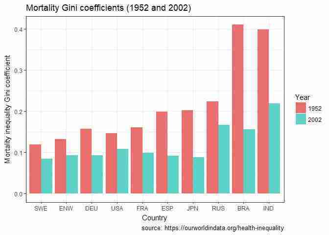
Mortality Gini coefficients (1952 and 2002).

Figure 5.10 Mortality Gini coefficients (1952 and 2002).

Now the country ordering is in terms of the average HGini, rather than HGini in 1952 (which might have made comparisons easier).

Note: Questions 3 and 4 can be done independently of each other.

Other measures of health inequality, such as those used by the World Health Organization (WHO), are based on access to healthcare, affordability of healthcare, and quality of living conditions. Choose one of the following measures of health inequality to answer Question 3:

access to essential medicines
basic hospital access
composite coverage index.

The composite coverage index is a weighted score of coverage for eight different types of healthcare.

To download the data for your chosen measure:

If you choose to look at either the access to essential medicines or the basic hospital access measure, go to the WHO’s Universal Health Coverage Data Portal, click on the tab ‘Explore UHC Indicators’, and select your chosen measure.
- A drop-down menu with three buttons will appear: ‘Map’ (or ‘Graph’) shows a visual description of the data, ‘Data’ contains the data files, and ‘Metadata’ contains information about your chosen measure.
- Click on the ‘Data’ button, then select ‘CSV table’ from the ‘Download complete data set as’ list.
If you choose to look at the composite coverage index measure, go to WHO’s Global Health Observatory data repository. The index is given for subgroups of the population, by economic status, education, and place of residence. Choose one of these categories, and download the data by clicking ‘CSV table’ from the ‘Download complete data set as’ list. You can read further information about this index in the WHO’s technical notes.

For your chosen measure:

Explain how it is constructed and what outcomes it assesses.

Create an appropriate chart to summarize the data for all available countries. (You can replicate a chart shown on the website or draw a similar chart.)

Explain what your chart shows about health inequality within and between countries, and discuss the limitations of using this measure (for example, measurement issues or other aspects of inequality that this measure ignores).

R walk-through 5.10 Drawing a column chart with sorted values

For this walk-through, we downloaded the ‘access to essential medicines’ data, as explained above. Here we saved it as WHO access to essential medicines.csv. Looking at the spreadsheet in Excel, you can see that the actual data starts in row three, meaning there are two header rows. So let’s skip the first row when uploading it.
med_access  read.csv(
  "WHO access to essential medicines.csv", skip = 1)
str(med_access)
## 'data.frame':  38 obs. of 3 variables:
##  $ Country     : Factor w/ 38 levels "Afghanistan",..: 1 2 3 4 5 6 7 8 9 10 ...
##  $ X2007.2013  : num  94 42.9 86.7 76.7 72.1 58.3 13.3 90.7 31.3 33.3 ...
##  $ X2007.2013.1: num  81.1 43.2 31.9 0 87.1 46.7 15.5 86.7 21.2 100 ...
Using the str function to inspect the dataset, you can see that the second and third variables have lost their labels during the import. From the spreadsheet you know that they are:

median availability of selected generic medicines (%) – Private

median availability of selected generic medicines (%) – Public.

Let’s change the names of these variables (to Private_Access and Public_Access respectively) to make working with them easier:
names(med_access)[2]  "Private_Access"
names(med_access)[3]  "Public_Access"
To find details about these variables, click the ‘Metadata’ button on the website to find the following explanation (under ‘Method of measurement’):

A standard methodology has been developed by WHO and Health Action International (HAI). Data on the availability of a specific list of medicines are collected in at least four geographic or administrative areas in a sample of medicine dispensing points. Availability is reported as the percentage of medicine outlets where a medicine was found on the day of the survey.

Before we produce charts of the data, we shall look at some summary measures of the access variable (med_access).
summary(med_access)
##                              Country   Private_Access   Public_Access   
##  Afghanistan                     : 1   Min.   :  2.80   Min.   :  0.00  
##  Bahamas                         : 1   1st Qu.: 54.62   1st Qu.: 39.67  
##  Bolivia (Plurinational State of): 1   Median : 70.15   Median : 55.95  
##  Brazil                          : 1   Mean   : 65.97   Mean   : 58.25  
##  Burkina Faso                    : 1   3rd Qu.: 86.70   3rd Qu.: 82.50  
##  Burundi                         : 1   Max.   :100.00   Max.   :100.00  
##  (Other)                         :32                    NA's   :2
On average, private sector patients have better access to essential medication.

From the summary statistics for the Public_Access variable, you can see that there are two missing observations (NA). Here, we will keep these observations because leaving them in doesn’t affect the following analysis.
med_access  med_access[complete.cases(med_access), ]
There are a number of interesting aspects to look at. We shall produce a bar chart comparing the private and public access in countries, ordered according to values of private access (largest to smallest). First, we need to reformat the data into ‘long’ format (so there is a single variable containing all the values we want to plot), then use the ggplot function to make the chart.
# Reorder by values of private access (largest to smallest)
med_access$Country  reorder(
  med_access$Country, med_access$Private_Access) 

# This is required for the melt function.
library(reshape2)
# Rearrange the data for ggplot
med_access_melt  melt(med_access)

# This creates a dataframe with three columns
# Country = Country name
# value = % access (Private_Access or Public_Access).
# variable = indicates Public_Access or Private_Access. 

ggplot(med_access_melt, 
  aes(x = Country, y = value, fill = variable)) +
  geom_bar(position = "dodge", stat = "identity") +
  scale_fill_discrete(name = "Access",
    labels = c("Private sector", "Public sector")) +
  theme(axis.text.x = element_text(angle = 90, 
    hjust = 1, vjust = 0.5)) +
  theme_bw() +
  labs(title = "Access to essential medication", 
    x = "Country", y = "Percent of patients with access to 
      essential medication") +
  # Flip axis to make country labels readable
  coord_flip()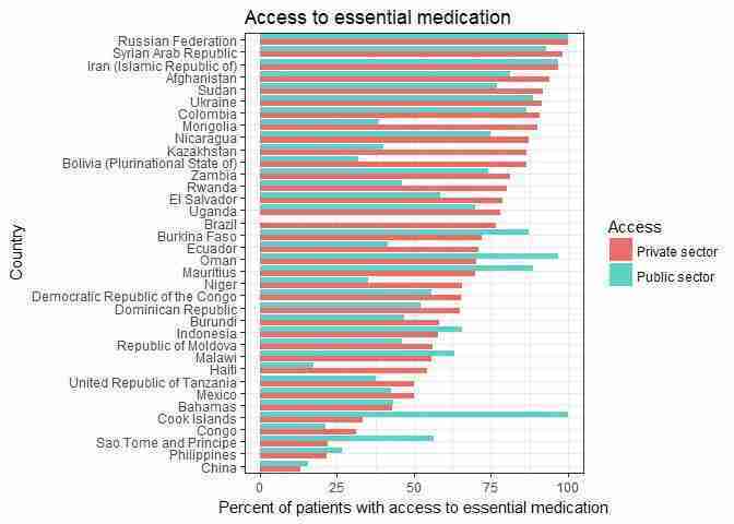
Access to essential medication.

Figure 5.11 Access to essential medication.

Let’s find the extreme values, starting with the two countries where public sector patients have access to all (100%) essential medications (which you can also see in the chart).
med_access[med_access$Public_Access == 100, ]
##               Country Private_Access Public_Access
## 10       Cook Islands           33.3           100
## 30 Russian Federation          100.0           100
Let’s see which countries provide 0% access to essential medication for people in the public sector.
med_access[med_access$Public_Access == 0, ]
##   Country Private_Access Public_Access
## 4 Brazil  76.7           0

Since an individual’s income and available options in later life partly depend on their level of education, inequality in educational access or attainment can lead to inequality in income and other outcomes. Gender inequality can be measured by the share of women at different levels of attainment. We will focus on the aspect of gender inequality in educational attainment, using data from the Our World in Data website, to make our own comparisons between countries and over time. Choose one of the following measures to answer Question 4:

gender gap in primary education (share of enrolled female primary education students)
share of women, between 15 and 19 years old, with no education
share of women, 15 years and older, with no education.

To download the data for your chosen measure:

Go to the ‘Educational Mobility and Inequality’ section of the Our World in Data website, and find the chart for your chosen measure.
Click the ‘Data’ button at the bottom of the chart, then click the blue button that appears to download the data in csv format.

For your chosen measure:

Choose ten countries that have data from 1980 to 2010. Plot your chosen countries on the same line chart, with year on the horizontal axis and share on the vertical axis. Make sure to include a legend showing country names and label the axes appropriately.

Describe any general patterns in gender inequality in education over time, as well as any similarities and differences between countries.

Calculate the change in the value of this measure between 1980 and 2010 for each country chosen. Sort these countries according to this value, from the smallest change to largest change. Now plot a column chart showing the change (1980 to 2010) on the vertical axis, and country on the horizontal axis. Add data labels to display the value for each country.

Which country had the largest change? Which country had the smallest change?

Suggest some explanations for your observations in Questions 4(b) and (d). (You may want to do some background research on your chosen countries.)

Discuss the limitations of using this measure to assess the degree of gender inequality in educational attainment and propose some alternative measures.

R walk-through 5.11 Using line and bar charts to illustrate changes in time

Import data and plot a line chart

First we import the data into R and check its structure.
# Open the csv file from the working directory
data_prim  read.csv(
  "OWID-gender-gap-in-primary-education.csv")
str(data_prim)
## 'data.frame':  8780 obs. of 4 variables:
##  $ Entity                                         : Factor w/ 250 levels "Afghanistan",..: 1 1 1 1 1 1 1 1 1 1 ...
##  $ Code                                           : Factor w/ 207 levels "","ABW","AFG",..: 3 3 3 3 3 3 3 3 3 3 ...
##  $ Year                                           : int  1970 1971 1972 1973 1974 1975 1976 1977 1978 1980 ...
##  $ Primary.education..pupils....female.....female.: num  14.1 13.7 14 14.5 14.4 ...
The data is now in the dataframe data_prim. The variable of interest (percentage of female enrolment) has a very long name so we will shorten it to PFE.
names(data_prim)[4]  "PFE"
As usual, ensure that you understand the definition of the variables you are using. In the Our World in Data website, look at the ‘Sources’ tab underneath the graph for a definition:

Percentage of female enrollment is calculated by dividing the total number of female students at a given level of education by the total enrolment at the same level, and multiplying by 100.

This definition implies that if the primary-school-age population was 50% male and 50% female and all children were enrolled in school, the percentage of female enrolment would be 50.

Before choosing ten countries, we check which countries (Entity) are in the dataset using the unique function. Here we also use the head() function to only show the first few countries.
head(unique(data_prim$Entity))
## [1] Afghanistan         Albania             Algeria            
## [4] Andorra             Angola              Antigua and Barbuda
## 250 Levels: Afghanistan Albania Algeria Andorra ... Zimbabwe
You can find nearly all the countries in the world in this list (plus some sub- and supra-country entities, like OECD countries, which explains why the variable wasn’t initially called ‘Country’).

Plot a line chart for a selection of countries

We now make a selection of ten countries. (You can of course make a different selection, but ensure that you get the spelling right as R is unforgiving!).
temp_data  subset(data_prim, Entity %in% c(
  "Albania", "China", "France", "India", "Japan", 
  "Switzerland", "United Arab Emirates", 
  "United Kingdom", "Zambia", "United States"))
Now we plot the data, similar to what we did earlier.
ggplot(temp_data, aes(x = Year, y = PFE, color = Entity)) +
  # size = 1 sets the line thickness.
  geom_line(size = 1) +
  # Remove grey background
  theme_bw() +   
  # Change the set of colours used
  scale_colour_brewer(palette = "Paired") + 
  scale_colour_discrete(name = "Country") +
  # Set the vertical axis label
  ylab("Percentage (%)") +
  # Add a title
  ggtitle("Female pupils as a percentage of 
    total enrolment in primary education")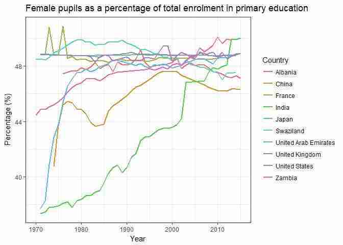 
Female pupils as a percentage of total enrolment in primary education.

Figure 5.12 Female pupils as a percentage of total enrolment in primary education.

Plot a column chart with sorted values

To calculate the change in the value of this measure between 1980 and 2010 for each country chosen, we have to manipulate the data so that we have one entry (row) for each entity (or country), but two different variables for the percentage of female enrolment PFE (one for each year).
# Select all data for 1980
temp_data_80  subset(temp_data, Year == "1980")
# Rename variable to include year
names(temp_data_80)[4]  "PFE_80"
# Select all data for 2010
temp_data_10  subset(temp_data, Year == "2010") 
# Rename variable to include year
names(temp_data_10)[4]  "PFE_10"
temp_data2  merge(
  temp_data_80, temp_data_10, by = c("Entity"))
Have a look at temp_data2, which now contains two variables for every country, PFE_80 and PFE_10. It also has multiple variables for Year (Year.x and Year.y) and Code (Code.x and Code.y), but that is a minor issue and you could delete one of them.

Now we can calculate the difference.
temp_data2$dPFE  temp_data2$PFE_10 - temp_data2$PFE_80
You could plot a separate chart for each year and check the order, but here we show how to create one chart with the data from both years.
ggplot(temp_data2, aes(
  x = reorder(Code.x, dPFE), y = dPFE)) +
  geom_bar(stat = "identity", fill = "tomato3") +
  labs(title = "Change (%) in female pupils’ share of 
    total enrolment in primary education",
    x = "Country", y = "Percentage change (%)",
    caption = "source: https://ourworldindata.org/educational-mobility-inequality") +
  theme_bw()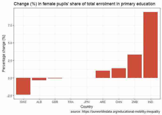
Change in percentage of female enrolment in primary school from 1980 to 2010.

Figure 5.13 Change in percentage of female enrolment in primary school from 1980 to 2010.

It is apparent that some countries saw very little or no change (the countries that already had very high PFE). The countries with initially low female participation have significantly improved.

University of Manchester’s Econometric Computing Learning Resource (ECLR). 2018. ‘R TSplots’. Updated 26 July 2016. ↩

Empirical Project 5 Working in R

Download the code

R-specific learning objectives

Getting started in R

Part 5.1 Measuring income inequality

Learning objectives for this part

R walk-through 5.1 Importing an Excel file (either `.xlsx` or .`xls` format) into R

R walk-through 5.2 Calculating cumulative shares using the `cumsum` function

R walk-through 5.3 Drawing Lorenz curves

R walk-through 5.4 Calculating Gini coefficients

Extension R walk-through 5.5 Calculating Gini coefficients for all countries and all years using a loop

Extension R walk-through 5.6 Plotting time series of Gini coefficients, using ggplot

Part 5.2 Measuring other kinds of inequality

Learning objectives for this part

R walk-through 5.7 Importing `.csv` files into R

Tip

R walk-through 5.8 Creating line graphs with `ggplot`

R walk-through 5.9 Drawing a column chart with sorted values

Plot a column chart for 1952

Plot a column chart for 2002

R walk-through 5.10 Drawing a column chart with sorted values

R walk-through 5.11 Using line and bar charts to illustrate changes in time

Import data and plot a line chart

Plot a line chart for a selection of countries

Plot a column chart with sorted values

Doing Economics

Empirical Project 5 Working in R

Download the code

R-specific learning objectives

Getting started in R

Part 5.1 Measuring income inequality

Learning objectives for this part

R walk-through 5.1 Importing an Excel file (either .xlsx or .xls format) into R

R walk-through 5.2 Calculating cumulative shares using the cumsum function

R walk-through 5.3 Drawing Lorenz curves

R walk-through 5.4 Calculating Gini coefficients

Extension R walk-through 5.5 Calculating Gini coefficients for all countries and all years using a loop

Extension R walk-through 5.6 Plotting time series of Gini coefficients, using ggplot

Part 5.2 Measuring other kinds of inequality

Learning objectives for this part

R walk-through 5.7 Importing .csv files into R

Tip

R walk-through 5.8 Creating line graphs with ggplot

R walk-through 5.9 Drawing a column chart with sorted values

Plot a column chart for 1952

Plot a column chart for 2002

R walk-through 5.10 Drawing a column chart with sorted values

R walk-through 5.11 Using line and bar charts to illustrate changes in time

Import data and plot a line chart

Plot a line chart for a selection of countries

Plot a column chart with sorted values

Doing Economics

R walk-through 5.1 Importing an Excel file (either `.xlsx` or .`xls` format) into R

R walk-through 5.2 Calculating cumulative shares using the `cumsum` function

R walk-through 5.7 Importing `.csv` files into R

R walk-through 5.8 Creating line graphs with `ggplot`