Empirical Project 7 Working in Excel
Part 7.1 Drawing supply and demand diagrams
Learning objectives for this part
- convert from the natural logarithm of a number to the number itself
- draw graphs based on equations.
- First download the data on the watermelon market. Read the Data dictionary tab and make sure you know what each variable represents.
- Download the paper ‘Suits’ Watermelon Model’ on the watermelon market.
The data is in natural logs: for example, the numbers in the price column are the logs of the prices of watermelons in each year, rather than the prices in dollars. Before plotting supply and demand curves we will first practise converting natural logarithms to numbers. In Part 7.2 we will discuss why it is useful to express relationships between variables (for example, price and quantity) in natural logs.
- To make charts that look like those in Figure 1 in the paper, you need to convert the relevant variables to their actual values. Excel’s EXP function does the inverse of the LN function, converting the natural log of a number to the number itself. (See Excel walk-through 4.3 for an example of the use of the LN function.)
- Create two new variables containing the actual values of P and Q.
- Plot separate line charts for P and Q, with time (in years) on the horizontal axis. Make sure to label your vertical axes appropriately. Your charts should look the same as Figure 1 in the paper.
Now we will plot supply and demand curves for a simplified version of the model given in the paper. We will define Q as the quantity of watermelons, in millions, and P as the price per thousand watermelons, and assume that the supply curve is given by the following equation:
Technical note
Whenever log (or ln) is used in economics, it refers to natural logarithms. Since this equation shows the price in terms of quantity (instead of quantity in terms of price), it is technically referred to as the inverse supply curve. However, we will be using the terms ‘supply curve’ and ‘demand curve’ to refer to both the supply/demand curve and the inverse supply/demand curve.
Using the same notation, the following equation describes the demand curve:
To plot a curve, we need to generate a series of points (vertical axis values that correspond to particular horizontal axis values) and join them up. First we will work with the variables in natural log format, and then we will convert them to the actual prices and quantities so that our supply and demand curves will be in familiar units.
- In a new tab on your spreadsheet:
- Create a table as shown in Figure 7.2. The first column contains values of Q from 20 to 100, in intervals of 5. (Remember that quantity is measured in millions, so Q = 20 corresponds to 20 million watermelons.)
| Q | Log Q | Supply (log P) | Demand (log P) | Supply (P) | Demand (P) |
|---|---|---|---|---|---|
| 20 | |||||
| 25 | |||||
| … | |||||
| 95 | |||||
| 100 |
Calculating supply and demand.
Figure 7.2 Calculating supply and demand.
- Convert the values of Q to natural log format (second column of your table) and use these values, along with the numbers in the equations above, to calculate the corresponding values of log P for supply (third column) and demand (fourth column).
- Use Excel’s EXP function to convert the log P values into the actual prices, P (fifth and sixth columns).
- Plot your calculated supply and demand curves on a line chart, with price (P) on the vertical axis and quantity (Q) on the horizontal axis. Make sure to label your curves (for example, using a legend).
- exogenous
- Coming from outside the model rather than being produced by the workings of the model itself. See also: endogenous.
During the time period considered (1930–1951), the market for watermelons experienced a negative supply shock due to the Second World War. Supply was limited because production inputs (land and labour) were being used for the war effort. This shock shifted the entire supply curve because the cause (Second World War) was not part of the supply equation, but was external (also known as being exogenous). Before doing the next question, draw a supply and demand diagram to illustrate what you would expect to happen to price and quantity as a result of the shock (all other things being equal). To see how oil shocks in the 1970s caused by wars in the Middle East shifted the supply curve in the oil market, see Section 7.13 in Economy, Society, and Public Policy.
Now we will use equations to show the effects of a negative supply shock on your Excel chart. Suppose that the supply curve after the shock is:
- Add the new supply curve to your line chart and interpret the outcomes, as follows:
- Create a new column in your table from Question 2 called ‘New supply (log P)’, showing the supply in terms of log prices after the shock. Make another column called ‘New supply (P)’ showing the supply in terms of the actual price in dollars.
- Add the New supply (P) values to your line chart and verify that your chart looks as expected. Make sure to label the new supply curve.
Consumer and producer surplus are explained in Sections 7.6 and 7.11 of Economy, Society, and Public Policy.
- From your chart, what can you say about the change in total surplus, consumer surplus, and producer surplus as a result of the supply shock? (Hint: You may find the following information useful: the old equilibrium point is Q = 64.5, P = 161.3; the new equilibrium point is Q = 55.0, P = 183.7).
Part 7.2 Interpreting supply and demand curves
Learning objectives for this part
- give an economic interpretation of coefficients in supply and demand equations
- distinguish between exogenous and endogenous shocks
- explain how we can use exogenous supply/demand shocks to identify the demand/supply curve.
You may be wondering why it is useful to express relationships in natural log form. In economics, we do this because there is a convenient interpretation of the coefficients: in the equation log Y = a + b log X, the coefficient b represents the elasticity of Y with respect to X. That is, the coefficient is the percentage change in Y for a 1 per cent change in X. To look at the concept of elasticity in more detail, see Section 7.8 of The Economy.
Supply curve:
Demand curve:
- Use the supply and demand equations from Part 7.1 which are shown here, and carry out the following:
- Calculate the price elasticity of supply (the percentage change in quantity supplied divided by the percentage change in price) and comment on its size (in absolute value). (Hint: You will have to rearrange the equation so that log Q is in terms of log P.)
- Calculate the price elasticity of demand in the same way and comment on its size (in absolute value).
Now we will use this information to take a closer look at the model of the watermelon market in the paper and interpret the equations.
The paper assumes that in practice farmers decide how many watermelons to grow (supply) based on last season’s prices of watermelons and other crops they could grow instead (cotton and vegetables), and the current political conditions that support or limit the amount grown. The reasoning for using last season’s prices is that watermelons take time to grow and are also perishable, so farmers cannot wait to see what prices will be in the next season before deciding how many watermelons to plant.
The estimated supply equation for watermelons is shown below (this is equation (1) in the paper):
- dummy variable (indicator variable)
- A variable that takes the value 1 if a certain condition is met, and 0 otherwise.
Here, C and T are the prices of cotton and vegetables, and CP is a dummy variable that equals 1 if the government cotton-acreage-allotment program was in effect (1934–1951). This program was intended to prevent cotton prices from falling by limiting the supply of cotton, so farmers who reduced their cotton production were given government compensation according to the size of their reduction. WW2 is a dummy variable that equals 1 if the US was involved in the Second World War at the time (1943–1946).
You can read more about the government farm programs for cotton during this time period on pages 67–69 of the report ‘The cotton industry in the United States’.
- exogenous
- Coming from outside the model rather than being produced by the workings of the model itself. See also: endogenous.
- endogenous
- Produced by the workings of a model rather than coming from outside the model. See also: exogenous
In this model, the dummy variables and the prices of other crops are exogenous factors that affect the decisions of farmers, and hence also affect the endogenous variables P and Q that are determined by the interaction of supply and demand. The supply curve (right-hand panel of Figure 7.3) shows that if the price rose with no change in exogenous factors, then the quantity supplied by farmers would rise, along the supply curve. But if there is an exogenous shock, captured by a dummy variable, it shifts the entire supply curve by changing its intercept (left hand panel). This changes the supply price for any given quantity. (In this specific example of watermelons, the vertical axis variable would be the log price in the previous period, and the horizontal axis variable would be the quantity in the current period).
Supply curve: Dummy variables shift the entire curve (left-hand panel) while changes in endogenous variables move along the curve (right-hand panel).
Figure 7.3 Supply curve: Dummy variables shift the entire curve (left-hand panel) while changes in endogenous variables move along the curve (right-hand panel).
- With reference to Figure 7.4, for each variable in the supply equation, give an economic interpretation of the coefficient (for example, explain the effect on the farmers’ supply decision) and (where relevant) relate the coefficient to an elasticity.
| Variable | Coefficient | 95% confidence interval |
|---|---|---|
| P (price of watermelons) | 0.580 | [0.572, 0.586] |
| C (price of cotton) | –0.321 | [–0.328, –0.314] |
| T (price of vegetables) | –0.124 | [–0.126, –0.122] |
| CP (cotton program) | 0.073 | [0.068, 0.077] |
| WW2 (Second World War) | –0.360 | [–0.365, –0.355] |
Supply equation coefficients and 95% confidence intervals.
Figure 7.4 Supply equation coefficients and 95% confidence intervals.
Now we will look at the demand curve (equation (3) in the paper). The paper specifies per capita demand () in terms of price and other variables. () is the demand curve intercept:
- Using the demand equation and Figure 7.5, give an economic interpretation of each coefficient and (where relevant) relate the coefficient to an elasticity.
| Variable | Coefficient | 95% confidence interval |
|---|---|---|
| P (price of watermelons) | –1.125 | [–1.738, –0.512] |
| Y/N (per capita income) | 1.750 | [0.778, 2.722] |
| F (railway freight costs) | –0.968 | [–1.674, –0.262] |
Demand equation coefficients and 95% confidence intervals.
Figure 7.5 Demand equation coefficients and 95% confidence intervals.
Earlier, we mentioned that exogenous supply/demand shocks shift the entire supply/demand curve, whereas endogenous changes (such as changes in price) result in movements along the supply or demand curve. Exogenous shocks that only shift supply or only shift demand come in handy when we try to estimate the shape of the supply and demand curves. Read the information on simultaneity below to understand why exogenous shocks are important for identifying the supply and demand curves.
- simultaneity
- When the right-hand and left-hand variables in a model equation affect each other at the same time, so that the direction of causality runs both ways. For example, in supply and demand models, the market price affects the quantity supplied and demanded, but quantity supplied and demanded can in turn affect the market price.
The simultaneity problem Why we need exogenous shocks that shift only supply or demand
In the model of supply and demand, the price and quantity we observe in the data are jointly determined by the supply and demand equations, meaning that they are chosen simultaneously. In other words, the market price affects the quantity supplied and demanded, but the quantity supplied and demanded can in turn affect the market price. In economics we refer to this problem as simultaneity. We cannot estimate the supply and demand curves with price and quantity data alone, because the right-hand-side variable is not independent, but is instead dependent on the left-hand-side variable.
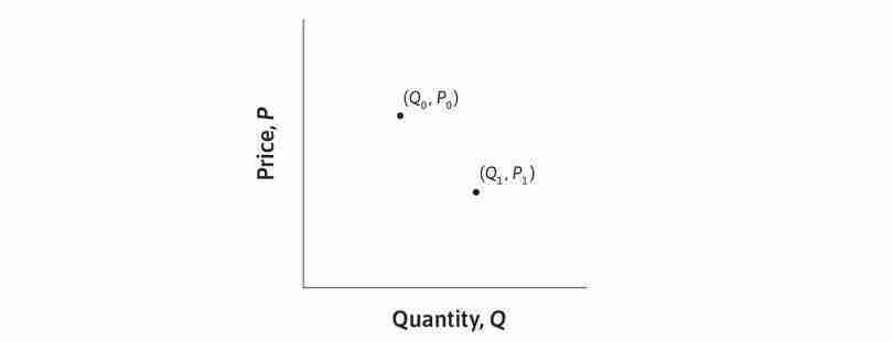
In the watermelon dataset, the price and quantity we observe for each year is the equilibrium of supply and demand in that year. The changes in the equilibrium from year to year happen as a result of both shifts and movements along the supply and demand curves, and we cannot disentangle these shifts or movements of the supply and demand curves without additional information. Figure 7.6 illustrates that there can be many different supply and demand curve shifts to explain the same data.
To address this issue, we need to find an exogenous variable that affects one equation but not the other. That way we can be sure that what we observe is due to a shift in one curve, holding the other curve fixed. In the watermelon market, we used the Second World War as an exogenous supply shock in Part 7.1. The war affected the amount of farmland dedicated to producing watermelons, but arguably did not affect demand for watermelons.
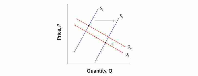
Figure 7.7 shows how we can use the exogenous supply shock to learn about the demand curve. The solid line shows the part of the demand curve revealed by the supply shock. Under the assumption that the demand curve is a straight line, we can infer what the rest of the curve looks like. If we had more information, for example if the size of the shock varied in each period, then we could use this information to learn more about the shape of the demand curve (for example, check whether it is actually linear). We use similar reasoning (exogenous demand shocks) to identify the supply curve.
- Given the supply and demand equations in the watermelon model, give two examples of an exogenous demand shock and explain why they are exogenous.
