Empirical Project 3 Solutions
These are not model answers. They are provided to help students, including those doing the project outside a formal class, to check their progress while working through the questions using the Excel, R, or Google Sheets walk-throughs. There are also brief notes for the more interpretive questions. Students taking courses using Doing Economics should follow the guidance of their instructors.
Part 3.1 Before-and-after comparisons of retail prices
-
Three Store Price Surveys (SPS) were conducted in a sample of stores to collect data on beverages, one before the tax was implemented, and two after. The sample of stores contains stores most visited by participants. To ensure that the sample is representative, additional stores within different categories of stores were added via random selection. Some selected stores refused to participate in the data collection, in which case randomly selected stores of the same type and neighbourhood were used as replacements.
A list of top-selling beverages was identified. Price data for each beverage was collected in each store by trained data collectors who followed standardized procedures. Some stores did not have any beverages in the list. Additional beverages similar to those in the list were therefore included in a supplementary panel.
Data were entered into a database using a tablet computer and paper forms. To avoid mistakes in transferring data from paper forms to the computer, the data on paper forms were double-entered. The two copies were compared and if results were dissimilar, the corresponding value in the paper forms was entered again.
- There are 247 different products in the dataset.
-
Solution figure 3.1 shows the frequency table for all store types in December 2014 and June 2015.
The number of observations for each store type is similar in each time period. Store type 4 is associated with the largest percentage change over time of about 32%.
| Store Type | Dec 2014 | Jun 2015 | Total |
|---|---|---|---|
| 1 | 177 | 209 | 386 |
| 2 | 407 | 391 | 798 |
| 3 | 87 | 102 | 189 |
| 4 | 73 | 96 | 169 |
| Grand total | 744 | 798 | 1,542 |
Frequency table: All stores in December 2014 and June 2015.
Solution figure 3.1 Frequency table: All stores in December 2014 and June 2015.
-
Solution figures 3.2 and 3.3 show the frequency tables for taxed and non-taxed beverages for December 2014 and June 2015 separately.
In both periods, the number of taxed and non-taxed beverages is similar for each store type.
| Store Type | No Tax | Tax | Total |
|---|---|---|---|
| 1 | 92 | 85 | 177 |
| 2 | 196 | 211 | 407 |
| 3 | 44 | 43 | 87 |
| 4 | 34 | 39 | 73 |
| Grand total | 366 | 378 | 744 |
Numbers of taxed and untaxed beverages by store type, December 2014.
Solution figure 3.2 Numbers of taxed and untaxed beverages by store type, December 2014.
| Store Type | No Tax | Tax | Total |
|---|---|---|---|
| 1 | 111 | 98 | 209 |
| 2 | 192 | 199 | 391 |
| 3 | 52 | 50 | 102 |
| 4 | 44 | 52 | 96 |
| Grand total | 399 | 399 | 798 |
Numbers of taxed and untaxed beverages by store type, June 2015.
Solution figure 3.3 Numbers of taxed and untaxed beverages by store type, June 2015.
-
Solution figure 3.4 shows the number of product types available in December 2014 and June 2015.
The SODA type has the highest number of observations. The SPORT-DIET type has the lowest number of observations.
Beverages belonging to more popular types are more likely to be in the panel of beverages. More popular types therefore tend to have more observations, since they are likely to be available in a greater number of stores.
| Row Labels | Dec 2014 | Jun 2015 | Total |
|---|---|---|---|
| Energy | 56 | 58 | 114 |
| Energy-diet | 49 | 54 | 103 |
| Juice | 70 | 64 | 134 |
| Juice Drink | 19 | 17 | 36 |
| Milk | 63 | 61 | 124 |
| Soda | 239 | 262 | 501 |
| Soda-diet | 128 | 174 | 302 |
| Sport | 11 | 16 | 27 |
| Sport-diet | 2 | 2 | 4 |
| Tea | 52 | 45 | 97 |
| Tea-diet | 6 | 6 | 12 |
| Water | 48 | 38 | 86 |
| Water-sweet | 1 | 1 | 2 |
| Grand total | 744 | 798 | 1,542 |
Product types available, December 2014 and June 2015.
Solution figure 3.4 Product types available, December 2014 and June 2015.
- Solution figure 3.5 shows the average price per oz (ounce) for taxed and non-taxed beverages.
| Non-taxed | Taxed | |||
|---|---|---|---|---|
| Store type | Dec 2014 | Jun 2015 | Dec 2014 | Jun 2015 |
| 1 | 11.19 | 11.48 | 15.62 | 16.93 |
| 3 | 15.20 | 16.08 | 18.18 | 19.08 |
Average price per ounce of taxed and non-taxed beverages, by time period and store type.
Solution figure 3.5 Average price per ounce of taxed and non-taxed beverages, by time period and store type.
-
Average prices increase over time for both types, whether taxed or not. This suggests that there is an upward time trend in prices that is independent of the tax.
For both groups, before the tax was implemented, the average price for the taxed (treatment) group is higher than that for the non-taxed (control) group. This suggests that the beverages subject to the tax were the more expensive beverages.
- No, because the difference in average price between the non-taxed group and the taxed group in any given period can be due to group-specific factors other than the tax. The difference in average price between the treatment and control groups in December 2014 before the implementation of the taxes suggests that the two groups are fundamentally different. The difference in June 2015 could be due to the differences between the groups rather than the taxes.
- Solution figure 3.6 shows the change in the mean price after the tax by store type.
| Non-taxed | Taxed | |
|---|---|---|
| Large supermarkets | 0.29 | 1.31 |
| Pharmacies | 0.88 | 0.90 |
Change in the mean price per oz ounce for taxed and non-taxed beverages, by store type.
Solution figure 3.6 Change in the mean price per oz ounce for taxed and non-taxed beverages, by store type.
- Solution figure 3.7 shows the mean change in price per oz for taxed and non-taxed beverages, by store type.
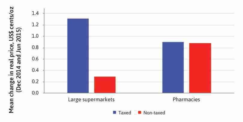
Mean change in price per oz for taxed and non-taxed beverages, by store type.
Solution figure 3.7 Mean change in price per oz for taxed and non-taxed beverages, by store type.
Note: When comparing these values to those in Silver et al. (2016), you will find that the data match for the ‘Large Supermarket’ and ‘Pharmacy store’ types, but not for the ‘Small Supermarket’ and ‘Gas Station store’ types. These discrepancies are due to the differences in categories used by Silver et al. (2016), for example, Silver et al. use ‘Independent corner stores and independent gas stations’ and ‘Small chain supermarkets and chain gas stations’ instead of ‘Small supermarkets’ and ‘Gas stations’.
-
The p-value for large supermarkets is quite small, indicating that the data is not compatible with the hypothesis that there are no differences in the populations (before- and after-tax prices), as long as other assumptions about the data (e.g. stores were really sampled at random) were correct. Thus it is likely that the sugar tax had some effect on prices.
On the other hand, the p-value for pharmacies is quite large, so there is reasonably strong evidence in favour of our assumption that there are no differences in the populations.
Part 3.2 Before-and-after comparisons with prices in other areas
-
Ideally, we would like the characteristics of the non-Berkeley stores to be the same as those of the Berkeley stores, so that patterns observed for the non-Berkeley stores can inform us about the patterns of Berkeley stores, if there had not been tax changes. If the two regions are sufficiently similar, then the differences in changes in the mean prices can be attributed to the tax policy.
The researchers chose suitable comparison stores, as the stores’ characteristics are very similar to those in Berkeley.
- Solution figure 3.8 indicates the average price in each month for taxed and non-taxed beverages, according to location.
| Non-taxed | Taxed | |||
|---|---|---|---|---|
| Year/Month | Berkeley | Non-Berkeley | Berkeley | Non-Berkeley |
| 2013 | ||||
| 1 | 5.72 | 5.35 | 8.69 | 7.99 |
| 2 | 5.81 | 5.37 | 8.66 | 8.19 |
| 3 | 5.86 | 5.42 | 8.82 | 8.19 |
| 4 | 5.86 | 5.65 | 9.02 | 8.25 |
| 5 | 5.83 | 5.21 | 8.73 | 7.81 |
| 6 | 5.79 | 5.06 | 8.61 | 7.46 |
| 7 | 5.97 | 5.15 | 8.32 | 7.27 |
| 8 | 5.90 | 5.14 | 8.92 | 7.57 |
| 9 | 5.91 | 5.15 | 9.13 | 7.90 |
| 10 | 5.87 | 5.24 | 9.10 | 7.85 |
| 11 | 6.08 | 5.37 | 9.23 | 8.07 |
| 12 | 6.09 | 5.34 | 9.06 | 7.89 |
| 2014 | ||||
| 1 | 6.12 | 5.37 | 8.98 | 8.00 |
| 2 | 6.20 | 5.53 | 9.20 | 7.95 |
| 3 | 6.47 | 5.84 | 9.53 | 8.17 |
| 4 | 6.38 | 5.80 | 9.64 | 8.35 |
| 5 | 6.52 | 5.73 | 9.66 | 8.50 |
| 6 | 6.56 | 5.80 | 9.19 | 8.11 |
| 7 | 6.48 | 5.59 | 9.29 | 8.24 |
| 8 | 6.37 | 5.66 | 9.34 | 8.10 |
| 9 | 6.65 | 5.84 | 9.32 | 8.60 |
| 10 | 6.38 | 5.60 | 9.48 | 8.58 |
| 11 | 5.85 | 5.65 | 8.03 | 8.47 |
| 12 | 6.19 | 5.52 | 9.67 | 8.53 |
| 2015 | ||||
| 1 | 6.41 | 5.85 | 10.02 | 8.82 |
| 2 | 6.39 | 5.66 | 9.24 | 8.49 |
| 3 | 6.51 | 5.71 | 10.02 | 8.82 |
| 4 | 6.48 | 5.83 | 10.38 | 8.76 |
| 5 | 6.64 | 5.82 | 10.34 | 8.94 |
| 6 | 6.64 | 5.83 | 10.42 | 8.69 |
| 7 | 6.37 | 5.73 | 10.58 | 8.90 |
| 8 | 6.45 | 5.69 | 11.10 | 9.03 |
| 9 | 6.51 | 5.67 | 10.44 | 8.71 |
| 10 | 6.54 | 5.67 | 10.70 | 8.79 |
| 11 | 6.67 | 5.85 | 10.71 | 8.98 |
| 12 | 6.56 | 5.76 | 10.54 | 8.59 |
| 2016 | ||||
| 1 | 6.58 | 5.87 | 10.57 | 8.96 |
| 2 | 6.55 | 5.76 | 10.81 | 8.73 |
| Grand total | 6.27 | 5.58 | 9.58 | 8.35 |
Average prices of taxed and non-taxed beverages in Berkeley vs non-Berkeley stores.
Solution figure 3.8 Average prices of taxed and non-taxed beverages in Berkeley vs non-Berkeley stores.
-
Solution figure 3.9 shows the average price per month for taxed and non-taxed beverages, according to location.
Non-taxed goods in Berkeley are more expensive than those outside Berkeley. The difference in prices before the tax indicates there are fundamental differences between the two regions irrespective of the tax policy. The difference stays roughly the same after the tax. This suggests that there were probably no other changes in the period that affected the difference in prices.
Taxed goods in Berkeley are more expensive than those outside Berkeley. The difference in prices increased after the tax was implemented (March 2015 onwards).
The prices of taxed goods and non-taxed goods in non-Berkeley regions have similar time trends. The time trends of goods in non-Berkeley regions are also similar to those in Berkeley. If we strip away the time trend, the prices of taxed and non-taxed goods in non-Berkeley regions remain roughly the same before and after the tax. This means that any events that took place during the period did not affect the level of prices in Berkeley and its neighbouring areas.
-
It is reasonable to conclude that the sugar tax had an effect on prices. The difference between the prices of the taxed goods in Berkeley and those outside Berkeley after the tax was implemented reflects both the effect of the tax and the effects of other differences between the two regions. The difference between the prices before the tax reflects the effects of differences other than the tax policy between the two regions. The difference in prices after the implementation of the tax, subtracting the difference in prices before the tax, gives us the effect of the tax. The increase in the difference in prices suggests that the tax has a positive effect on prices.
Note: When you compare this figure to Figure 3 in the Silver et al. paper you will notice that it is somewhat different. The effect of the tax is much more clearly visible in the paper. The reason for this difference is that the authors adjusted the prices for a number of factors (for example, see the notes to Figure 3) before they created the line chart. The adjustment process they used, however, is beyond the scope of this project.
-
The difference between the mean Berkeley and non-Berkeley price of non-sugary beverages after the tax reflects the effect of being in Berkeley as opposed to being in non-Berkeley regions. The difference between the mean Berkeley and non-Berkeley price of sugary beverages after the tax reflects not only the effect of being in Berkeley but also the effect of the tax. The difference in differences is the effect of the tax.
Based on the p-value, we can be reasonably confident in our assumption that the mean Berkeley and non-Berkeley prices of non-sugary beverages after the tax (in the population) are the same. In other words, there is reasonably strong evidence in favour of our assumption that there are no differences in the population means of these two groups.
The p-value for sugary drinks, however, is small, implying that it is quite unlikely to see the sample differences we see (or more extreme ones) if in truth there were no differences.
As we come to different conclusions about the after-tax price differences in drinks, this evidence is consistent with the hypothesis that the tax had an effect on sugary drinks prices.
-
Except for caloric intake of non-taxed beverages, the p-values of the other entries are fairly large. This implies that the differences in consumption behaviour we observe are likely to have occurred even if, in truth, there was no difference (the null hypothesis being no difference).
Beverages form a small proportion of the total budget of consumers. Consumers are unlikely to change their consumption by much given the tiny effect the price rise has on their budgets.
The two major ingredients in sugary beverages, water and sugar, are craved by the human body due to their importance for survival. Beverage companies have devoted tremendous efforts to make their beverages attractive to consumers. Many beverages have become part of people’s daily routines and have also become viewed as necessities for certain occasions. These factors mean that the demand for sugary beverages is price inelastic (not responsive to price changes).
People take time to change their consumption habits. Consumption patterns may change slowly over a long period of time. We need data for later periods to study the long-term effect of the tax.
-
Some of the limitations listed in the paper are:
- The study cannot fully distinguish the effect of the tax from the effect of other events, such as political campaigns related to the tax, which took place over the same period. The study cannot therefore establish the ceteris paribus causal effect of the tax. A more distant control (for example, another location that was not subject to these events) could be used to capture better the combined effects of the events and the tax.
- The study cannot tell whether the changes in behaviours were due to anticipation of the tax or changes in prices and sales.
- The sample of stores is too small and not representative. Consumption of SSB is small and the effect size is small relative to the high standard error. Future studies should use larger and more representative samples.
- There are limitations in the data from independently-owned small corner stores. The possible effect of shifts in purchases to these stores cannot be studied using the data in the study.
- A tax change could be implemented unexpectedly to reduce the effects of events such as campaigns in the periods of observation and to prevent behaviours from adjusting even before the experiment begins. If possible, ensure that there are no other policy changes that could affect the outcomes in the observation period. Also ensure that the treatment and control groups stay the same over the period, for example, by preventing the relocation of stores in response to the tax change. If possible, it is also important to prevent people from the taxed area from going to the neighbouring area to buy sugary drinks (which would be contrary to the purpose of the tax). Listing these factors helps to clarify the difficulties involved in establishing the conditions for a clean natural experiment in the real-world setting of policy implementation. In most countries, for example, it is not possible to prevent the relocation of stores and it would not be desirable to do so.
