Empirical Project 4 Solutions
These are not model answers. They are provided to help students, including those doing the project outside a formal class, to check their progress while working through the questions using the Excel, R, or Google Sheets walk-throughs. There are also brief notes for the more interpretive questions. Students taking courses using Doing Economics should follow the guidance of their instructors.
Note
These solutions are based on data downloaded in January 2018. Your solutions may differ slightly if using more updated data.
Part 4.1 GDP and its components as a measure of material wellbeing
- As the actual solution table is very long, only the first and last 10 rows are provided here, in Solution figure 4.1.
| Country | Number of years of GDP data |
|---|---|
| Afghanistan | 47 |
| Albania | 47 |
| Algeria | 47 |
| Andorra | 47 |
| Angola | 47 |
| Anguilla | 47 |
| Antigua and Barbuda | 47 |
| Argentina | 47 |
| Armenia | 27 |
| Aruba | 47 |
| … | … |
| Vanuatu | 47 |
| Venezuela (Bolivarian Republic of) | 47 |
| Viet Nam | 47 |
| Yemen | 28 |
| Yemen Arab Republic (Former) | 21 |
| Yemen Democratic (Former) | 21 |
| Yugoslavia (Former) | 21 |
| Zambia | 47 |
| Zanzibar | 27 |
| Zimbabwe | 47 |
Number of years of GDP data available for each country (1970–2016).
Solution figure 4.1 Number of years of GDP data available for each country (1970–2016).
- 179 out of 220 countries have data for the entire period. We have missing data from 19% of countries. Countries with missing data may have distinct characteristics compared with other countries. For example, poorer countries do not have the resources to collect data. It is therefore likely that for some years, the data available will be for an unrepresentative sample of countries.
- No solution is provided.
- This example uses China and the US.
- No solution is provided.
- Solution figures 4.2 and 4.3 show the value of the four components of GDP for the US and for China.
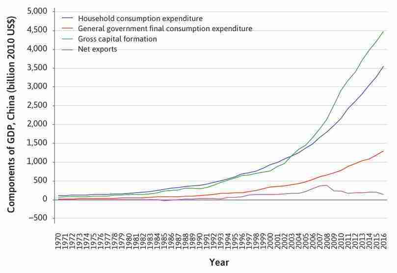
China’s GDP components (expenditure approach), 1970–2016.
Solution figure 4.3 China’s GDP components (expenditure approach), 1970–2016.
- For countries that are growing, consumption expenditures and capital formation can be increasing together as the additional income is split between them. This pattern is shown in both countries in the period before the global financial crisis in 2008. In the data for the US, investment expenditure and consumption fall markedly in the financial crisis and both government spending and net export expenditure move in the opposite direction. (If you are interested in understanding what lies behind these patterns, see Units 13 and 14 in The Economy.) Note also that China’s net exports fall markedly during the global financial crisis: this does not reflect changes in the Chinese economy, but the fall in expenditure in China’s major trading partners, including the US.
-
China’s economic growth started to accelerate in the late 1970s due to a stream of reforms to promote marketization, privatization, openness to trade, and other objectives. The government shifted the priority of its development strategies away from capital-intensive heavy industries and towards labour-intensive manufacturing industries that take better advantage of China’s abundance of labour. In December 2001, China joined the World Trade Organization, which accelerated its integration into the world economy. China’s comparative advantage in manufacturing due to its abundant and cheap labour has contributed to the rapid growth of net exports which remain a key driver of China’s growth today. The rapid economic growth has allowed all three components to increase simultaneously. The decentralization and the declining role of state-owned enterprises have contributed to the decreasing relative size of government expenditure.
The United States, as a developed economy, has been growing at relatively slow rates between 1970 and 2016. The net exports component has been decreasing as production of many goods has moved to low-cost developing countries. Most of the gains in income are devoted to household consumption, which has been rising at a disproportionately high rate compared with the other components.
From the charts, the most obvious difference between China and the US lies in the relative importance of capital formation, that is, investment expenditure on machinery, equipment, and buildings, including infrastructure. In particular, while capital formation is the largest component in China, it is a relatively small component in the US. In fact, capital formation in the US is only about one third of household consumption.
- An example for China is shown in Solution figure 4.4.
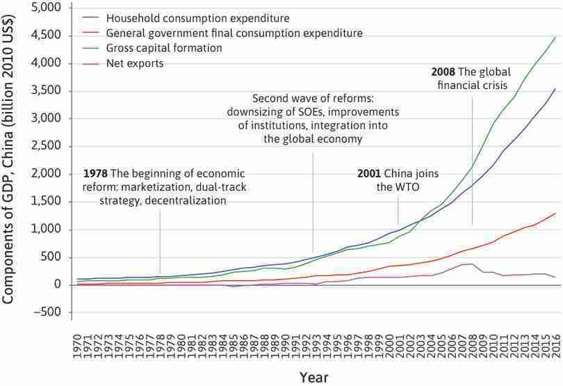
China’s GDP components (expenditure approach), with annotations (1970–2016).
Solution figure 4.4 China’s GDP components (expenditure approach), with annotations (1970–2016).
- China and the US are used as examples.
- No solution is provided.
- Solution figures 4.5 and 4.6 show the proportion of the component of GDP by year for China and for the US.
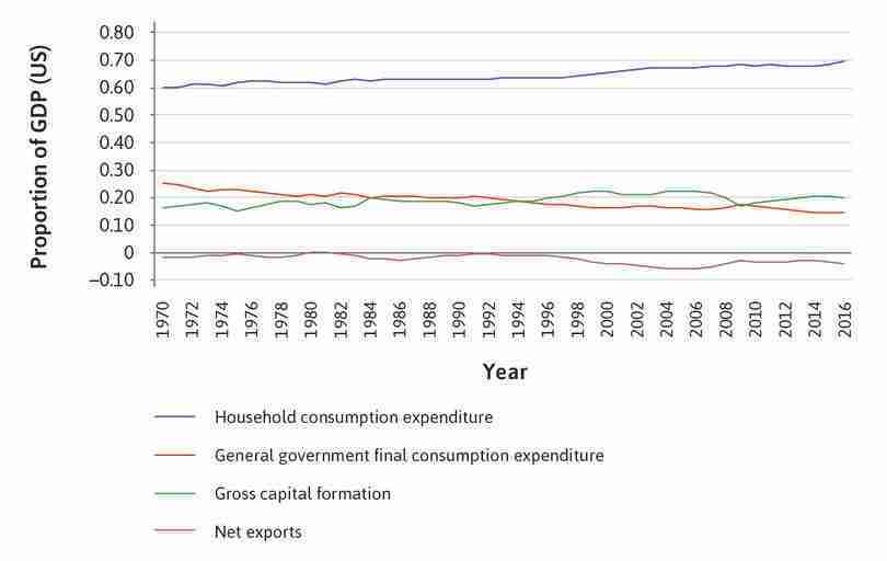
Share of components of GDP in the US (1970–2016).
Solution figure 4.6 Share of components of GDP in the US (1970–2016).
-
In China, household consumption accounted for 56% of GDP in 1970 but has since fallen to a low point of 36% in 2010, after which it stabilized. It was 37% in 2016. The share of capital formation fluctuated around 37% between 1970 and 2000. After 2000, capital formation experienced a period of rapid increase, reaching 48% in 2010 before stabilizing. The share of government consumption is relatively small, about 10% in 1970, and has been increasing slowly, reaching 14% in 2016. The net exports component was negative and decreasing prior to 1986. After 1986, net exports increased rapidly, reaching 8% of GDP in 2008, before remaining relatively stable.
In the US, household consumption remains the largest component throughout the period, and increased from 60% in 1970 to 70% in 2016. Capital formation fluctuates without a clear trend. Government consumption fell from 25% in 1970 to 14% in 2016. The net exports component is negative and has been falling slightly.
While the share of household consumption has been falling in China, it has been increasing in the US. Capital formation is relatively small in comparison to household consumption in the US. In China, however, capital formation rose more rapidly and in 2003 surpassed household consumption to become the largest component of GDP. While the share of government consumption in China has no clear trend, it has been falling in the US.
-
It is difficult to tell the relative proportions (and thus the importance) of each component from the charts in Question 3, which are plotted using levels. The charts of levels show that the governments have been growing in size. When we look at the charts of proportions, we realize that the proportion of government consumption expenditure in the US has been falling, and has no clear trend in China.
The charts in levels are more difficult to compare across countries because countries have different income levels. The charts of proportions have common units and bounds and are therefore easier for cross-country comparisons.
-
The following countries are used as examples:
- developing economies: Brazil, China, India
- economies in transition: Albania, Russian Federation, Ukraine
- developed countries: Germany, Japan, United States.
- Solution figure 4.7 provides the calculation for each component as a proportion of GDP for 2015.
| Country | Indicator name | Proportion of GDP |
|---|---|---|
| Brazil | Household consumption expenditure | 0.64 |
| Brazil | General government final consumption expenditure | 0.19 |
| Brazil | Gross capital formation | 0.17 |
| Brazil | Net exports | 0.00 |
| China | Household consumption expenditure | 0.37 |
| China | General government final consumption expenditure | 0.13 |
| China | Gross capital formation | 0.47 |
| China | Net exports | 0.02 |
| India | Household consumption expenditure | 0.55 |
| India | General government final consumption expenditure | 0.10 |
| India | Gross capital formation | 0.36 |
| India | Net exports | −0.01 |
| Albania | Household consumption expenditure | 0.78 |
| Albania | General government final consumption expenditure | 0.11 |
| Albania | Gross capital formation | 0.27 |
| Albania | Net exports | −0.16 |
| Russian Federation | Household consumption expenditure | 0.52 |
| Russian Federation | General government final consumption expenditure | 0.17 |
| Russian Federation | Gross capital formation | 0.20 |
| Russian Federation | Net exports | 0.11 |
| Ukraine | Household consumption expenditure | 0.69 |
| Ukraine | General government final consumption expenditure | 0.22 |
| Ukraine | Gross capital formation | 0.16 |
| Ukraine | Net exports | −0.07 |
| Germany | Household consumption expenditure | 0.55 |
| Germany | General government final consumption expenditure | 0.19 |
| Germany | Gross capital formation | 0.19 |
| Germany | Net exports | 0.07 |
| Japan | Household consumption expenditure | 0.57 |
| Japan | General government final consumption expenditure | 0.20 |
| Japan | Gross capital formation | 0.24 |
| Japan | Net exports | 0.00 |
| United States | Household consumption expenditure | 0.62 |
| United States | General government final consumption expenditure | 0.13 |
| United States | Gross capital formation | 0.19 |
| United States | Net exports | 0.07 |
Share of each component of GDP for a selection of countries in 2015.
Solution figure 4.7 Share of each component of GDP for a selection of countries in 2015.
- Solution figure 4.8 shows the composition of GDP in 2015 by country.
- Developing countries spend less on household consumption and more on capital formation compared to the other two types of countries. The proportion of income spent on government consumption tends to be higher in developed countries.
-
GDP per capita is the total value of all output (and thus income) in an economy divided by the population in a period of time. GDP per capita is by definition a measure of material wellbeing. The measure is based on the assumption that market prices of goods and services are good indicators of the amount of welfare they bring to economic agents. GDP per capita is relatively straightforward to calculate and use. GDP per capita is also a relatively objective measure. GDP per capita is the most widely-used measure and huge resources have been devoted to establishing the infrastructure for its computation.
Even as a measure of material wellbeing, GDP per capita has limitations:
- Goods and services such as caring for family relatives are not accounted for by GDP per capita because they are not traded in markets and hence do not have prices. GDP per capita understates material wellbeing for this reason.
- Economic activities that produce pollution are included in GDP but the detriment they cause to material wellbeing is not. GDP per capita overstates material wellbeing for this reason.
- Income generated by production in a country may not remain in that country or get used by people living in the country. Some of the income may be appropriated by foreign companies repatriating profits from their affiliates. The measure gross national income per capita adjusts for this.
- GDP per capita is an average across the population and therefore does not reflect the inequality in material wellbeing within the country. A country can have a high GDP per capita while having income concentrated in a narrow section of the population.
- There is a wide scope for different answers here using the two sources listed as well as material in Section 4.14 of Economy, Society, and Public Policy.
Part 4.2 The HDI as a measure of wellbeing
-
There are many valid points that can be made about the suitability of these measures, for example:
The gross national income of a country consists of its GDP, plus income earned by residents living in foreign countries, minus income earned domestically by non-residents. GNI per capita, despite having many limitations, is the best widely available measure of living standards we have.
The expected years of schooling and mean years of schooling are not good measures of knowledge. Most importantly, the quality of education varies across countries.
Life expectancy, especially in developing countries, can be driven by rapid changes in infant and child mortality, and therefore may fail to reflect longevity. A longer life does not necessarily mean a healthy life.
These indicators all have limitations as measures of the relevant dimensions.
-
There are many possible answers, for example:
These values are completely reasonable. Starvation, diseases, land erosion, and the lack of incentives are day-to-day realities for the people of the poorest countries in the world. Due to low income, poor countries cannot afford healthcare and education. Poor healthcare and education, many economists argue, may be the cause of low income in the first place.
- (a)–(c) No solution is provided. For (b), if education is missing for one of the education variables, take the value of the available index as the education index.
- No solution is provided.
- For the indicators in this example, child malnutrition and mortality rate (male and female) are used for health. Adult literacy rate, tertiary enrolment, and primary school teachers trained to teach are used for education.
-
Child malnutrition has a major impact on the welfare of children and on their physical and cognitive development. Child malnutrition is therefore a good indicator of the future health of children when they grow up and hence a good indicator of the health of the population.
The mortality rate is driven by health. Although mortality rate is a determinant of life expectancy, the measure does not involve forming expectations of how long someone will live.
The quantity of education can be a poor indicator of knowledge due to the varying quality of education across countries. Furthermore, most countries, including developing countries, have achieved very high primary and secondary enrolment rates, resulting in less variation across countries.
The adult literacy rate is by definition a measure that better reflects the stock of knowledge in the economy. Primary school teachers trained to teach is a good and available measure of the quality of education.
Tertiary education is typically financed by individuals rather than by governments. As a result, there is great variation across countries in tertiary enrolment. Universities, unlike primary and secondary schools, play a major role in pushing the frontier of research and innovation.
- The respective min and max functions were used to determine a reasonable minimum and maximum value for each indicator in Solution figure 4.9.
| Indicator | Minimum | Maximum |
|---|---|---|
| Child malnutrition (% under age 5) | 1.30 | 57.50 |
| Female mortality rate (per 1,000 people) | 32.24 | 612.37 |
| Male mortality rate (per 1,000 people) | 63.70 | 580.50 |
| Adult literacy rate (% ages 15 and older) | 19.13 | 99.89 |
| Tertiary Enrolment (% of tertiary school-age population) | 0.80 | 110.16 |
| Primary school teachers trained to teach (% of primary school teachers) | 5.86 | 100.00 |
Minimum and maximum values of the chosen indicators.
Solution figure 4.9 Minimum and maximum values of the chosen indicators.
Note that the tertiary enrolment can be greater than 100% due to students in tertiary education who are younger or older than the usual age at which people receive tertiary education (18–23 years old).
-
The alternative HDI can only be calculated for a limited number of countries that have full data for all the variables chosen. When choosing the indicators, missing data did not seem to be an issue, as only a few countries lack data for each particular indicator. However, the set of countries lacking data for one or more of the indicators turns out to be large.
The missing data problem is more common among the richest countries. For example, adult literacy rate is missing for Norway, Australia, US, UK, and other European countries (though this information can be found from other data sources, such as the CIA Factbook).
- Missing data means that the alternative HDI was available for only 80 countries. As shown in Solution figure 4.10, countries with higher HDI tend to have higher alternative HDI. There are, however, exceptions. Columbia, for example, ranked 24 out of the 80 countries in terms of HDI, is ranked 10 in terms of alternative HDI. Swaziland, ranked 51 out of 80 in HDI, is ranked 70 in alternative HDI.
| Country | Alternative Health index | Alternative Education index | Alternative Income index | Alternative HDI excluding countries with missing data | Alternative HDI rank | HDI rank |
|---|---|---|---|---|---|---|
| Brunei Darussalam | 0.866 | 0.702 | 0.996 | 0.846 | 3 | 1 |
| Saudi Arabia | 0.905 | 0.828 | 0.943 | 0.891 | 1 | 2 |
| Kuwait | 0.936 | 0.658 | 1.002 | 0.851 | 2 | 3 |
| Belarus | 0.820 | 0.932 | 0.763 | 0.836 | 4 | 4 |
| Kazakhstan | 0.724 | 0.804 | 0.815 | 0.780 | 9 | 5 |
| Malaysia | 0.812 | 0.728 | 0.832 | 0.789 | 8 | 6 |
| Panama | 0.809 | 0.728 | 0.796 | 0.777 | 14 | 7 |
| Costa Rica | 0.926 | 0.795 | 0.747 | 0.819 | 6 | 8 |
| Serbia | 0.888 | 0.677 | 0.726 | 0.758 | 19 | 9 |
| Cuba | 0.914 | 0.788 | 0.651 | 0.777 | 13 | 10 |
| Iran (Islamic Republic of) | 0.922 | 0.811 | 0.770 | 0.832 | 5 | 11 |
| Georgia | 0.853 | 0.763 | 0.677 | 0.761 | 17 | 12 |
| Sri Lanka | 0.807 | 0.627 | 0.707 | 0.710 | 29 | 13 |
| Lebanon | 0.895 | 0.759 | 0.739 | 0.795 | 7 | 14 |
| Mexico | 0.848 | 0.717 | 0.770 | 0.776 | 15 | 15 |
| Azerbaijan | 0.796 | 0.732 | 0.770 | 0.766 | 16 | 16 |
| Algeria | 0.863 | 0.669 | 0.741 | 0.754 | 22 | 17 |
| Armenia | 0.794 | 0.718 | 0.665 | 0.724 | 26 | 18 |
| Ukraine | 0.793 | 0.914 | 0.649 | 0.778 | 12 | 19 |
| Thailand | 0.777 | 0.810 | 0.752 | 0.779 | 11 | 20 |
| Ecuador | 0.762 | 0.700 | 0.704 | 0.721 | 27 | 21 |
| Mongolia | 0.734 | 0.853 | 0.702 | 0.761 | 18 | 22 |
| Jamaica | 0.869 | 0.687 | 0.668 | 0.736 | 24 | 23 |
| Colombia | 0.816 | 0.792 | 0.732 | 0.780 | 10 | 24 |
| Tunisia | 0.884 | 0.695 | 0.699 | 0.754 | 21 | 25 |
| Dominican Republic | 0.823 | 0.722 | 0.732 | 0.758 | 20 | 26 |
| Belize | 0.732 | 0.528 | 0.650 | 0.631 | 40 | 27 |
| Uzbekistan | 0.721 | 0.690 | 0.612 | 0.673 | 34 | 28 |
| Moldova (Republic of) | 0.814 | 0.765 | 0.592 | 0.717 | 28 | 29 |
| Botswana | 0.508 | 0.696 | 0.753 | 0.643 | 37 | 30 |
| Paraguay | 0.823 | 0.725 | 0.665 | 0.735 | 25 | 31 |
| Egypt | 0.748 | 0.562 | 0.697 | 0.664 | 35 | 32 |
| Palestine, State of | 0.875 | 0.785 | 0.598 | 0.743 | 23 | 33 |
| Viet Nam | 0.794 | 0.734 | 0.601 | 0.705 | 30 | 34 |
| Philippines | 0.629 | 0.758 | 0.669 | 0.683 | 33 | 35 |
| El Salvador | 0.753 | 0.689 | 0.657 | 0.698 | 32 | 36 |
| Kyrgyzstan | 0.766 | 0.703 | 0.519 | 0.653 | 36 | 37 |
| Morocco | 0.861 | 0.625 | 0.646 | 0.703 | 31 | 38 |
| Guyana | 0.736 | 0.547 | 0.639 | 0.636 | 39 | 39 |
| Tajikistan | 0.707 | 0.744 | 0.492 | 0.637 | 38 | 40 |
| Bhutan | 0.608 | 0.523 | 0.644 | 0.589 | 44 | 41 |
| Congo | 0.615 | 0.539 | 0.605 | 0.585 | 45 | 42 |
| Lao People's Democratic Republic | 0.566 | 0.628 | 0.592 | 0.595 | 43 | 43 |
| Bangladesh | 0.694 | 0.397 | 0.530 | 0.527 | 52 | 44 |
| Ghana | 0.649 | 0.455 | 0.551 | 0.546 | 49 | 45 |
| Sao Tome and Principe | 0.729 | 0.369 | 0.517 | 0.518 | 53 | 46 |
| Cambodia | 0.656 | 0.619 | 0.518 | 0.595 | 42 | 47 |
| Nepal | 0.652 | 0.547 | 0.476 | 0.554 | 46 | 48 |
| Myanmar | 0.612 | 0.675 | 0.589 | 0.624 | 41 | 49 |
| Pakistan | 0.603 | 0.469 | 0.592 | 0.551 | 47 | 50 |
| Swaziland | 0.193 | 0.555 | 0.653 | 0.412 | 70 | 51 |
| Angola | 0.472 | 0.390 | 0.626 | 0.486 | 58 | 52 |
| Tanzania (United Republic of) | 0.540 | 0.591 | 0.484 | 0.537 | 50 | 53 |
| Cameroon | 0.442 | 0.522 | 0.508 | 0.490 | 57 | 54 |
| Zimbabwe | 0.418 | 0.576 | 0.418 | 0.465 | 63 | 55 |
| Mauritania | 0.685 | 0.453 | 0.538 | 0.551 | 48 | 56 |
| Madagascar | 0.501 | 0.236 | 0.390 | 0.359 | 77 | 57 |
| Rwanda | 0.549 | 0.549 | 0.420 | 0.502 | 55 | 58 |
| Comoros | 0.596 | 0.511 | 0.391 | 0.492 | 56 | 59 |
| Lesotho | 0.152 | 0.523 | 0.529 | 0.348 | 78 | 60 |
| Senegal | 0.714 | 0.398 | 0.470 | 0.511 | 54 | 61 |
| Uganda | 0.479 | 0.552 | 0.425 | 0.482 | 59 | 62 |
| Sudan | 0.563 | 0.474 | 0.551 | 0.528 | 51 | 63 |
| Togo | 0.571 | 0.472 | 0.383 | 0.469 | 62 | 64 |
| Benin | 0.563 | 0.343 | 0.451 | 0.443 | 65 | 65 |
| Malawi | 0.485 | 0.493 | 0.359 | 0.441 | 66 | 66 |
| Côte d'Ivoire | 0.396 | 0.403 | 0.522 | 0.436 | 67 | 67 |
| Gambia | 0.598 | 0.434 | 0.413 | 0.475 | 60 | 68 |
| Ethiopia | 0.546 | 0.462 | 0.411 | 0.470 | 61 | 69 |
| Mali | 0.521 | 0.264 | 0.468 | 0.401 | 71 | 70 |
| Congo (Democratic Republic of the) | 0.489 | 0.572 | 0.289 | 0.433 | 69 | 71 |
| Liberia | 0.571 | 0.329 | 0.290 | 0.379 | 75 | 72 |
| Eritrea | 0.448 | 0.493 | 0.408 | 0.448 | 64 | 73 |
| Mozambique | 0.318 | 0.477 | 0.362 | 0.380 | 74 | 74 |
| Guinea | 0.548 | 0.322 | 0.356 | 0.398 | 72 | 75 |
| Burundi | 0.362 | 0.591 | 0.292 | 0.397 | 73 | 76 |
| Burkina Faso | 0.549 | 0.364 | 0.413 | 0.435 | 68 | 77 |
| Chad | 0.382 | 0.304 | 0.452 | 0.374 | 76 | 78 |
| Niger | 0.542 | 0.159 | 0.330 | 0.305 | 79 | 79 |
| Central African Republic | 0.334 | 0.263 | 0.267 | 0.286 | 80 | 80 |
Comparing alternative HDI rank and HDI rank.
Solution figure 4.10 Comparing alternative HDI rank and HDI rank.
- The same countries used in Question 5 are used as examples.
-
The classification of Belize and Uzbekistan changes from High human development to Medium human development.
Bangladesh, Ghana, and Sao Tome and Principe change from Medium human development countries to Low human development countries under the alternative HDI.
- Despite using very different indicators for health and education, the rank and classifications of countries under the alternative HDI are similar to those under HDI. HDI is therefore a robust measure of non-material wellbeing.
- Solution figure 4.11 provides the scatterplot for each country’s GDP per capita rank and HDI rank.
- There appears to be a strong correlation, because GDP per capita is a component of HDI. In addition, GDP per capita is strongly related to health and education, the other two components of HDI. We would therefore expect that GDP per capita and HDI would be strongly correlated.
- There are many possible ways to define ‘high’ GDP per capita; here we define ‘high’ as greater than 11,048 USD, the median of the group, as shown in Solution figure 4.12.
| HDI | |||
|---|---|---|---|
| Low | High | ||
| GDP per capita | Low | Afghanistan Zimbabwe Yemen |
Georgia Sri Lanka Albania |
| High | Botswana Iraq South Africa |
Norway Switzerland United States |
Comparison of countries according to GDP per capita and HDI.
Solution figure 4.12 Comparison of countries according to GDP per capita and HDI.
- GDP per capita measures the total value of all output in the economy per head of the population. HDI is a geometric mean of three dimension indices: health, education, and the natural log of income per capita. Unlike GDP per capita, the HDI takes into account the possibility that income might have diminishing marginal utility (that is, doubling your income might less than double your wellbeing). GDP per capita, however, assumes that wellbeing increases one-for-one with income, and that income is the only factor that determines wellbeing, which is not the case.
-
There are many possible strengths and weaknesses, including the following:
- Strengths: The HDI as a measure of wellbeing is more comprehensive than GDP per capita because it accounts for education and health outcomes. The HDI is widely used and recognized.
- Weaknesses: As mentioned before, schooling years and life expectancy may not be good indicators of knowledge and health, respectively. The three dimensions receive equal weight in HDI. Countries may have different views about which dimension is more important.
-
There are many possible measures, including the following:
- Unemployment affects people’s non-material wellbeing. Unemployed people often have no income except benefits, and are more likely to feel detached from the world and unhappy. Long-term unemployment could make it more and more difficult for people to be re-employed. The unemployment rate is measured as the percentage of the economically-active population that is out of work but is actively seeking work. For more discussion of these issues see Unit 8 of Economy, Society, and Public Policy on the labour market and unemployment, and Empirical Project 8, which investigates the non-monetary cost of unemployment.
- Inequality affects people’s satisfaction. It matters whether people get equal opportunities to succeed. People’s happiness may depend more on their relative income compared to that of others rather than the absolute value of income. Inequality measures such as the Gini coefficient and health inequality Gini coefficient can be used alongside HDI.
- There are many subjective measures of non-material wellbeing, such as gross national happiness and gross national wellbeing. These measures rely on surveys that ask people about their non-material wellbeing directly.
