8 The labour market and the product market: Unemployment and inequality
8.1 Introduction
- By putting the labour market and the product market together in a single model, we have a way to understand how unemployment and inequality are determined in the economy as a whole.
- The labour market functions quite differently from the bread market, described in the previous unit, because firms cannot purchase the work of employees directly but only hire their time.
- In modern economies, most product markets—also unlike the bread market—are dominated by large firms that face downward-sloping demand curves. These so-called ‘monopolistic competitors’ can control the prices at which their goods sell, and they set prices to maximize their profits.
- The outcome of the wage-setting process across all firms in the economy is the wage-setting curve, which shows for each unemployment rate the lowest wage that will motivate employees to work.
- The outcome of the price-setting process across all firms is the price-setting curve, which gives the value of the real wage that is consistent with the level of productivity and the extent of competition in markets for goods and services.
- The wage-setting and price-setting curves together determine the structural unemployment in the economy.
- The level of structural unemployment can be altered by public policies that change the productivity of labour, the degree of competition facing firms in product markets, the extent and nature of labour unions and labour law, and the unemployment benefit.
- Changes in how the labour and product markets function alter the distribution of income as measured by the Lorenz curve and the Gini coefficient.
- The model of the whole economy—product and labour market together—helps to explain how the growing monopoly power of firms has contributed to rising inequality in the US economy.
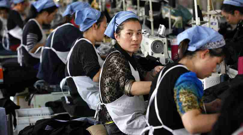
Mining was not a job, it was a way of life for Doug Grey, a rigger who operated giant cranes at mines in the Northern Territory, Australia. In the 1990s, he helped construct the MacArthur River zinc mine, one of the world’s largest, where his son Rob got his first job. ‘I ended up driving ore trucks,’ Rob recalled, ‘that was an awesome opportunity.’
Rob, it seemed then, had been born at the right time. He entered the labour market just as the worldwide natural resources boom was taking off, driven by the demand from China’s rapidly growing economy. Rob lived in Thailand for a time, spending little. He would take a flight to his job in Borroloola, a round trip of 10,000 km.
At about the time that Rob started work, Doug, the elder Grey, took a job at the Pilbara iron ore mine in Western Australia, which paid about twice the average family income in Australia at the time. Both father and son were putting away substantial savings.
But by 2015, the natural resource boom was a distant memory, and the price of ore and zinc continued to plummet. Rob and his fellow miners were worried. ‘Everybody knew the economic downturn and commodity prices were a problem. We had that in the back of our minds.’ Their dream economy couldn’t last. ‘It was … obvious … that it was coming to an end,’ Doug said.
And it did. In late 2015, Rob got the bad news: ‘Two days into my break the general manager called and said, “Thanks for your service, we appreciate it, we have to let you go.”’ His father, too, was laid off.
Driving ore trucks is Rob’s passion and he still hopes to get back behind the wheel. But that is not going to happen, at least not at the Pilbara mine where his dad once worked. Faced with collapsing demand, the mining company cut production, and also sought to drastically reduce costs. As part of this process, the company replaced human labour with machines wherever possible. In the Pilbara mine, nobody is behind the wheel of any of their giant robot ore trucks that are now being ‘driven’ by university graduates with joysticks 1,200 km away in Perth.
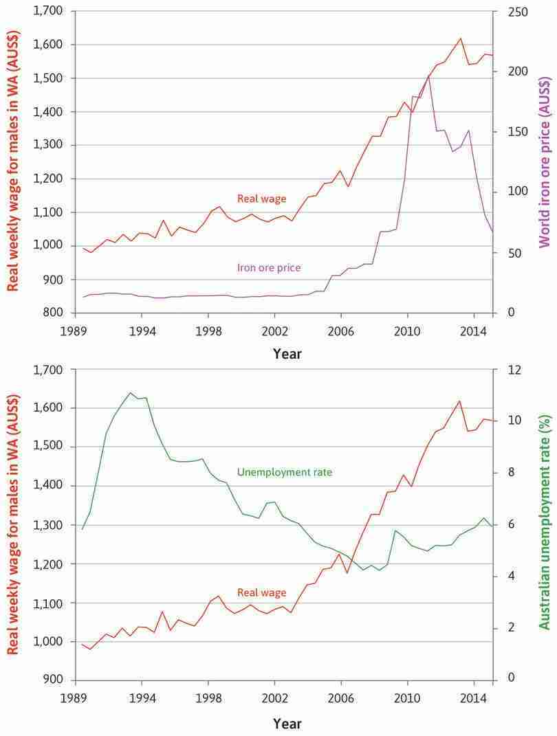
The rise and fall of the Grey family’s economic fortunes is an example of the workings of the labour market in the mining and construction industries in Western Australia and the Northern Territory. Figure 8.1 shows that their experience was far from unusual. The boom in ore prices (in the top figure) made mining highly profitable, leading to strong demand for labour, which eventually dried up the pool of unemployed riggers and truck drivers. Mining companies had no choice but to pay extraordinarily high salaries, and while the mining boom lasted, the companies remained highly profitable.
The downturn in commodity prices began in mid-2011 and unemployment began to rise. Born-at-the-right-time Rob Grey’s luck had run out.
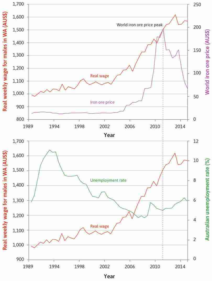
Real weekly earnings for males in Western Australia (left-hand axis), world price of iron ore and unemployment rate in Australia (right-hand axis), (1989–2015).
Figure 8.1 Real weekly earnings for males in Western Australia (left-hand axis), world price of iron ore and unemployment rate in Australia (right-hand axis), (1989–2015).
Australian Bureau of Statistics and International Monetary Fund. Note: Unemployment rates are seasonally adjusted.
Weekly earnings
The chart shows real weekly earnings for males in Western Australia, together with the world price of iron ore in the top panel and the unemployment rate in Australia in the bottom panel. As the unemployment rate dropped from 1994, real wages began to grow rapidly.
Figure 8.1a The chart shows real weekly earnings for males in Western Australia, together with the world price of iron ore in the top panel and the unemployment rate in Australia in the bottom panel. As the unemployment rate dropped from 1994, real wages began to grow rapidly.
Australian Bureau of Statistics and International Monetary Fund. Note: Unemployment rates are seasonally adjusted.
Growth slows, unemployment rises
Following the peak in iron ore prices, unemployment began to rise and real wage growth slowed.
Figure 8.1b Following the peak in iron ore prices, unemployment began to rise and real wage growth slowed.
Australian Bureau of Statistics and International Monetary Fund. Note: Unemployment rates are seasonally adjusted.
We learn from the patterns in the Australian labour market that wages increase when unemployment falls. From Unit 6, we know that firms have to set higher wages to ensure that employees work hard and well when unemployment in the economy is low. And from Unit 6, we also know that there will always be more people seeking jobs than the number of jobs offered. These are the involuntarily unemployed.
The model we develop in this unit helps to explain why, over very long periods, unemployment rates differ between countries. Take, for example, two large European countries, Germany and Spain. These countries share many characteristics. As well as belonging to the European Union, which provides conditions for borderless trade, firms based in both countries compete in global markets on the same terms. They share access to the same robot technologies and other labour-saving innovations.
The two countries appear to be equally vulnerable to what are generally considered to be the two potential ‘job killers’ for the high-income countries in the early twenty-first century—automation and globalization. Yet, for the period from 1960 to 2018, the unemployment rate in Germany averaged 5.5%, compared with a rate more than double this in Spain (13.8%).
The comparison of Spain and Germany directs attention to the contrasting ways in which both labour and product markets work in different countries. The model of the economy as a whole we develop in this unit helps to explain these differences, and how they can lead to different outcomes for unemployment and inequality. This information in turn can be the basis of more effective policies to sustain high wages and employment, and to limit the extent of inequality.
- unemployment
- A situation in which a person who is able and willing to work is not employed.
- population of working age
- A statistical convention, which in many countries is all people aged between 15 and 64 years.
- labour force
- The number of people in the population of working age who are, or wish to be, in work outside the household. They are either employed (including self-employed) or unemployed. See also: unemployment rate, employment rate, participation rate.
- inactive population
- People in the population of working age who are neither employed nor actively looking for paid work. Those working in the home raising children, for example, are not considered as being in the labour force and therefore are classified this way.
- participation rate
- The ratio of the number of people in the labour force to the population of working age. See also: labour force, population of working age.
8.2 Measuring the economy: Employment and unemployment
What does it mean to say that the unemployment rate was 13.8% in Spain and 5.5% in Germany? What exactly is ‘unemployment’?
According to the standardized definition of the International Labour Organization (ILO), the unemployed are the people who:
- were without work during a reference period (usually four weeks); in other words, they were not in paid employment or self-employment
- were available for work
- were seeking work; in other words, they had taken specific steps in that period to seek paid employment or self-employment.
Figure 8.2 provides an overview of the labour market and shows how these components fit together. We begin on the left-hand side, with the population. The next box shows the population of working age. This is the total population, minus children and those over 64. It is divided into two parts: the labour force and those out of the labour force (known as the inactive population). People out of the labour force are not employed or actively looking for work, for example, people unable to work due to sickness or disability, students, or parents who stay at home to raise children. Only members of the labour force can be considered as employed or unemployed.
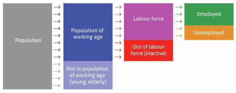
The labour market.
Figure 8.2 The labour market.
There are a number of statistics that are useful for evaluating labour market performance in a country and for comparing labour markets between countries. The statistics depend on the relative sizes of the boxes shown in Figure 8.2.
Participation rate
The first is the participation rate, which shows the proportion of the working-age population that is in the labour force. It is calculated as follows:
Unemployment rate
- unemployment rate
- The ratio of the number of the unemployed to the total labour force. (Note that the employment rate and unemployment rate do not sum to 100%, as they have different denominators.) See also: labour force, employment rate.
- employment rate
- The ratio of the number of employed to the population of working age. See also: population of working age.
Next is the most commonly cited labour market statistic—the unemployment rate. This shows the proportion of the labour force that is unemployed. It is calculated as follows:
Employment rate
Lastly, we come to the employment rate, which shows the proportion of the population of working age that are in paid work or self-employed. It is calculated as follows:
It is important to note that the denominator (the statistic on the bottom of the fraction) is different for the unemployment and the employment rate. Hence, two countries with the same unemployment rate can differ in their employment rates if one has a high participation rate and the other has a low one.
Comparing labour markets
The table in Figure 8.3 provides a picture of the labour markets in four countries—Australia, Germany, Norway, and Spain—between 2000 and 2016, and shows how the labour market statistics relate to each other.
It also shows that the structure of the labour market differs widely among different countries. We can see that the Norwegian labour market worked better than the Spanish labour market in the last 17 years—Norway had a much higher employment rate and a much lower unemployment rate. Norway also had a higher participation rate, which is a reflection of the higher proportion of women in the labour force.
| Australia | Germany | Norway | Spain | |
|---|---|---|---|---|
| Number of persons, millions | ||||
| Population of working age | 17.2 | 69.6 | 3.5 | 37.6 |
| Labour force | 11.1 | 41.0 | 2.5 | 21.6 |
| Out of labour force (inactive) | 6.1 | 28.5 | 1.0 | 16.0 |
| Employed | 10.5 | 38.0 | 2.4 | 18.1 |
| Unemployed | 0.6 | 3.1 | 0.1 | 3.5 |
| Rates (%) | ||||
| Participation rate | 11.1/17.2 = 65% |
41.0/69.6 = 59% |
2.5/3.5 = 71% |
21.6/37.6 = 58% |
| Employment rate | 10.5/17.2 = 61% |
38.0/69.6 = 55% |
2.4/3.5 = 69% |
18.1/37.6 = 48% |
| Unemployment rate | 0.6/11.1 = 6% |
3.1/41.0 = 7% |
0.1/2.5 = 4% |
3.5/21.6 = 16% |
Labour market statistics for Australia, Germany, Norway, and Spain (averages over 2000–2016).
Figure 8.3 Labour market statistics for Australia, Germany, Norway, and Spain (averages over 2000–2016).
International Labour Organization. 2018. ILOSTAT Database.
Norway and Spain are illustrations of two common cases. Norway is a low-unemployment, high-employment economy (the other Scandinavian countries—Sweden, Denmark, and Finland—are similar; and in the table, Australia is the country most similar to Norway). Spain is a high-unemployment, low-employment economy (the other southern European economies—Portugal, Italy and Greece—are other examples). Other combinations are possible, however—Germany’s participation rate is low like Spain’s but its unemployment and employment rate performance are much better.
Exercise 8.1 Using Excel: Employment, unemployment, and participation
- Visit the ILO’s website and use the ILOSTAT Database to calculate the average employment, unemployment, and participation rates over the period 2000–2016, for two economies of your choice.
- Create appropriate chart(s) to display these statistics for the countries in Figure 8.3 and your chosen countries. Using your chart(s), describe the similarities and differences in these statistics.
- After studying this unit, use the model of the labour market to suggest possible reasons for the differences in unemployment rates in these countries. You may need to find out more about the labour markets in your chosen countries.
Question 8.1 Choose the correct answer(s)
Which of the following statements are correct?
- Participation rate = labour force ÷ population of working age.
- Unemployment rate = unemployed ÷ labour force.
- This is the definition of the employment rate.
- Unemployment rate = unemployed ÷ labour force, while employment rate = employed ÷ population of working age. They do not add up to 1 because the denominator is different.
8.3 The labour market, the product market and the aggregate economy: The WS/PS model
To see why, over the long run, some countries (like Spain) have had much higher unemployment rates than others (like Germany), we will set out a model for an entire economy. This is referred to as a model of the aggregate economy or the macroeconomy. Economists use the term aggregate (meaning ‘whole’) to describe economy-wide facts or variables, like the labour market statistics in the previous section.
The same model will be used in Section 8.9 to show what happens when there is a change in the monopoly power of firms over time. This has happened in the past 30 years, for example, with the growth in market power of large firms in the technology sector.
The actors in the labour market include the employees, and the owners or managers of each firm. But within the management of the firm, there are two distinct actors: the human resources department (‘HR’) is in charge of setting wages to ensure that employees ‘work’, while the marketing department is tasked with setting a price that will maximize the firm’s profits.
We give the actors in our model these names, and imagine them in different departments, because this clarifies two different decisions taken in the operation of a firm. In reality, HR and marketing departments influence these decisions, but do not make them.
The model of the aggregate economy has two parts:
- The labour market: In which the focus is the relationship between employers and workers and on how wages are set by HR.
- The product market: In which the focus is the relationship between firms and their customers and on how prices are set by the marketing department.
Putting them together for all firms gives us a model of the aggregate economy.
- From the labour market, we get the wage-setting (WS) curve: For every level of employment it gives the real wage that HR would like to pay.
- From the product market, we get the price-setting (PS) curve: It tells us the real wage that results from the price-setting decisions of Marketing.
Where the two curves intersect shows the level of employment (and unemployment) and the real wage for which the decisions of the two departments are consistent. This is the equilibrium of the whole economy; you can think of it as a situation in which both Marketing and HR in all firms are satisfied.
- WS/PS model
- Model of the aggregate economy that combines wage-setting (WS) and price-setting (PS) decisions. Where the WS and PS curves intersect is the Nash equilibrium and determines structural unemployment and the real wage. See also, wage-setting curve, price-setting curve, structural unemployment.
We call the two curves—the wage-setting (WS) curve and the price-setting (PS) curve—including the reasoning behind them, the model of the aggregate economy. And we refer to it by its nickname, the WS/PS model.
8.4 The labour market and the wage-setting curve (firms and workers)
We started with the labour market and the fact that Rob Grey and his father—the Australian miners—did well while the economy was booming, earning high wages and having little fear of unemployment, and not so well when the economy hit the doldrums.
We generalize their experience in Figure 8.4, where the horizontal axis represents the proportion of the working-age population and goes up to a value of 1. The vertical axis is the economy-wide real wage.
- The labour force is the vertical line furthest to the right: It has a value less than 1, depending on the participation rate.
- Inactive workers are to the right of the labour force line.
- The employment rate is the vertical line to the left of the labour force, indicating the share of the population who are actually working.
- The unemployment rate is the proportion of those in the labour force who are not employed: that is, those workers in between the employment rate line and the labour force line.
- wage-setting (WS) curve
- The curve—arising from the wage-setting decisions of firms in the labour market—that gives the real wage necessary at each level of economy-wide employment to provide workers with incentives to work hard and well.
- worker’s best response function (to wage)
- The amount of work that a worker chooses to perform as her best response to each wage that the employer may offer. Also known as: best response curve.
The upward-sloping line is called the wage-setting (WS) curve. The wage-setting curve for the whole economy is based directly on the employer’s wage-setting decision and the employee’s effort decision in an economy that is composed of many firms, like the economy we modelled in Unit 6.
Follow the analysis in Figure 8.4 to understand the upward-sloping wage-setting curve. We focus on two specific rates of unemployment—5% and 12%—but there is nothing special about these numbers. They are purely illustrative.
The wage-setting (WS) curve: Labour discipline and unemployment in the economy as a whole.
Figure 8.4 The wage-setting (WS) curve: Labour discipline and unemployment in the economy as a whole.
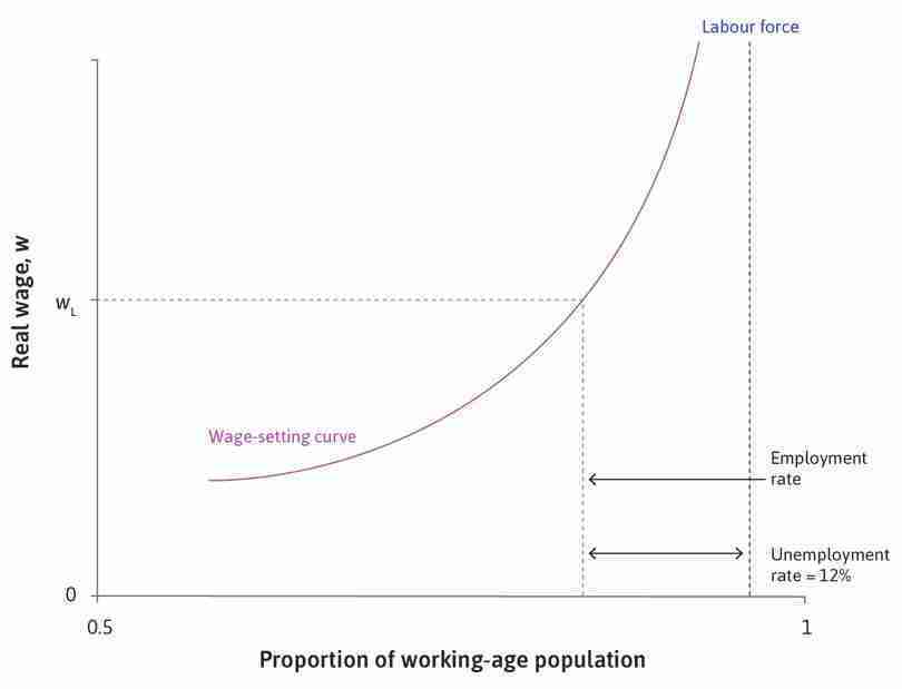
The wage set by firms when unemployment is high
At a relatively high unemployment rate (we chose 12%) in the economy, the employee’s reservation wage is low and they will put in high effort for a relatively low wage. Therefore, the firm’s chosen wage is low.
Figure 8.4b At a relatively high unemployment rate (we chose 12%) in the economy, the employee’s reservation wage is low and they will put in high effort for a relatively low wage. Therefore, the firm’s chosen wage is low.
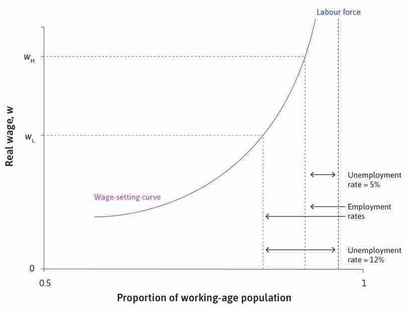
The wage set by firms when unemployment is low
At a relatively low unemployment rate (in this case, 5%) in the economy, the employee’s reservation wage is high and they will not put in adequate effort unless the wage is high. Therefore, the firm’s chosen wage is higher.
Figure 8.4c At a relatively low unemployment rate (in this case, 5%) in the economy, the employee’s reservation wage is high and they will not put in adequate effort unless the wage is high. Therefore, the firm’s chosen wage is higher.
Employment, unemployment, and out of the labour force
The right-most dotted blue line shows the total working-age population, which is divided into the employed, the unemployed, and those not participating in the labour force.
Figure 8.4d The right-most dotted blue line shows the total working-age population, which is divided into the employed, the unemployed, and those not participating in the labour force.
Figure 8.5 brings together Figure 8.4 (the economy-wide wage-setting curve) and Figure 6.7 (how the firm sets the wage). The top panel of Figure 8.5 shows the employee’s best response curve at the two unemployment rates of 12% and 5%. The same analysis applies to any other unemployment rate you wish to choose.
As we saw in Unit 6, a higher unemployment rate reduces the reservation wage, because a worker faces a longer expected period of unemployment if they lose a job. This weakens the bargaining power of the employee and shifts the best response curve to the left. With an unemployment rate of 12%, the reservation wage is shown by point F. The employer’s profit-maximizing choice is point A with the low wage (wL).
In the lower panel, we plot point A on the wage-setting curve. The dashed line from an unemployment rate of 12% indicates that the wage is set at wL. We assume a fixed size for the labour force and the horizontal axis gives the number of workers employed, N. As employment increases to the right, the unemployment rate falls.
Using exactly the same reasoning, we find the profit-maximizing wage set when unemployment is 5%. Both the reservation wage and the wage set by the employer are higher, as shown by point B. This gives the second point on the wage-setting curve in the lower panel.
When Rob and Doug Grey write their biography, they will label point B as a Golden Age, early in this century, when Rob was living in Thailand and flying to his job at Borroloola, and his father was operating giant cranes at the Pilbara mine. Point A is Paradise Lost, after the minerals boom ended.
- labour discipline model
- A model that explains how employers set wages so that employees receive an economic rent (called employment rent), which provides workers an incentive to work hard in order to avoid job termination. See also: employment rent, efficiency wages.
We derived the wage-setting curve as part of the labour discipline model, which was designed to illustrate how employees and employers interact when setting wages and determining the level of work effort. We will use the same model when we describe government policies to alter the level of unemployment in the entire economy. Later in this unit, we will look at the ways in which labour unions can affect the wage-setting process and so alter the workings of the labour market.
Real wages and nominal wages
- real wage
- The nominal wage, adjusted to take account of changes in prices between different time periods. It measures the amount of goods and services the worker can buy. See also: nominal wage.
- consumer price index (CPI)
- A measure of the general level of prices that consumers have to pay for goods and services, including consumption taxes.
When the employer sets the wage, it is set in nominal terms, that is in euros, dollars, or pesos, for example. But workers care about what they can buy with their wages. They care about the real wage, which is written as w = W/P, where P is the price level in the economy. The price level is constructed by combining the prices of the goods and services in a typical basket of goods consumed by the worker. An example of a price level is the consumer price index (CPI). Throughout the analysis of the interaction between the employee and employer in wage-setting, we use the real wage, w, because it is the real wage that motivates the worker to work hard.
The wage-setting curve for the US economy
Figure 8.6 is a wage-setting curve estimated from data for the US. Note that, in Figure 8.6, the horizontal axis shows the unemployment rate explicitly, falling from left to right. On the vertical axis is the real wage, measured by real annual earnings. By using data on unemployment rates and wages in local areas, economists can estimate and plot the wage-setting curve for an economy.
Wage-setting curves have been estimated for many economies. David Blanchflower and Andrew Oswald explain how it is done in their paper ‘The Wage Curve’.
A wage-setting curve estimated for the US economy (1979–2013).
Figure 8.6 A wage-setting curve estimated for the US economy (1979–2013).
Estimated by Stephen Machin (UCL, 2015) from Current Population Survey microdata from the Outgoing Rotation Groups for 1979 to 2013.
Simplifying the model
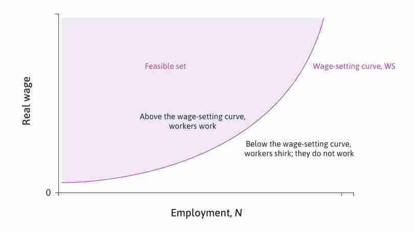
We can simplify the worker motivation problem and the wage curve by letting there be just two levels of effort:
- ‘working’: providing the level of effort that the firm’s owners and managers have set as sufficient
- ‘shirking’: providing no effort at all.
This will be useful later because it will allow us to take the level of effort as given with wages being set to ensure this.
In this case, the worker is represented as similar to a machine with just one speed, and it is either ‘on’ or ‘off’. As shown in Figure 8.7, the wage curve is the boundary between two ‘regions’: on and above the wage curve are all the combinations of the real wage and employment level for which employees work, and below it the combinations for which employees shirk.
The wage-setting curve: The wage level required to make employees work rather than shirk.
Figure 8.7 The wage-setting curve: The wage level required to make employees work rather than shirk.
We will use this ‘work or shirk’ simplification in the model from now on.
What shifts the wage-setting curve?
- employment rent
- The economic rent a worker receives when the net value of her job exceeds the net value of her next best alternative (that is, being unemployed). Also known as: cost of job loss.
What determines the height of the wage-setting curve? In Unit 6, we studied the determinants of the cost of job loss. For any unemployment rate, a change in any of the elements raising the employment rent a worker gets from their job shifts the wage-setting curve downwards, as shown in the table in Figure 8.8.
For example, because a lower unemployment benefit makes it more costly if you lose your job, your employment rent is higher and the firm can set a lower wage and you will work, rather than shirk. Another example is an increase in the labour force. If there are more people searching for jobs, then you can expect to remain without work for longer if you lose your job. This increases the rents you get from your current job and shifts the wage-setting curve downwards.
A new technology that allows easier monitoring of shirking (such as the use of GPS trackers in trucks, monitoring their location at any time) makes detection of shirking less costly; the firm can set a lower wage and the worker will work rather than shirk. The wage-setting curve shifts downwards.
Exercise 8.2 Shifts in the wage-setting curve
- Referring back to Unit 6, provide a brief explanation of the shift in the wage-setting curve for each row in Figure 8.8, using a diagram to show the best response function and the wage-setting curve. For the second and third rows, give an example from a real-world workplace.
- Explain why a rise in the unemployment rate shifts the best response function but not the wage-setting curve.
Change Shifts the wage-setting curve Decrease in unemployment benefit Down Increase in social stigma attached to being unemployed Down A decrease in the disutility of working Down Shifts in the wage-setting curve.
Figure 8.8 Shifts in the wage-setting curve.
Question 8.2 Choose the correct answer(s)
Figure 8.5 depicts the wage-setting curve and how it is derived using the best response function of the employees and the isocost lines for effort of the employers.
Based on this figure:
- A cut in the unemployment benefit would shift the best response function to the left. However, this would mean that the equilibrium wage falls for a given unemployment rate and lowers the wage-setting curve.
- An extended expected unemployment period would shift the best response function to the left, lowering the wage-setting curve.
- If there is high stigma attached to unemployment, then the workers’ best response functions would move to the left. This reduces the equilibrium wage for a given unemployment rate, resulting in a lower wage-setting curve.
- With the balance of job seekers and vacancies shifting in favour of the workers, their best response function would shift to the right, resulting in the wage-setting curve moving upwards.
8.5 The product market and the price-setting curve (firms and customers)
- price-setting (PS) curve
- The curve—arising from the price-setting decisions of firms in markets for goods and services (the product market)—that gives the real wage paid when firms choose their profit-maximizing price.
The wage-setting curve alone does not fix the level of employment in the model—the economy could be at any combination of employment and the real wage along it. To pin this down, we need to bring in the market for goods and services, the product market, and another curve, the price-setting (PS) curve.
It gets its name because it gives the real wage that is the outcome of the choice by the firm’s marketing department of a profit-maximizing price for their products. We will see how this price-setting curve is determined just below; but first we explain how bringing together the labour market and the product market in the WS and PS curves provides the information we need to determine the wage and employment level in the economy.
The two curves intersect at the real wage and level of employment (and the associated rate of unemployment) the economy can sustain. It is an equilibrium in the labour market and in the product market because:
- If the economy is on the wage-setting curve, workers won’t shirk: At this rate of unemployment, this is the real wage at which workers will provide adequate effort and production can take place.
- If the economy is on the price-setting curve, then given their costs and the markup, firms are setting their profit-maximizing price: The result of that decision is a real wage shown by the price-setting curve.
When the economy is at the intersection of the wage- and price-setting curves, employees provide adequate effort and firms are willing to employ that number of workers because, given the demand they face for their output and their costs, the firms are setting their profit-maximizing price.
- structural unemployment
- The level of unemployment at the Nash equilibrium of the labour and product market model.
This is what is called the structural unemployment, because it is the equilibrium level of unemployment determined by the two curves, representing the structure of the economy: profit-maximizing price-setting by firms in product markets, and profit-maximizing wage-setting by firms in labour markets. Structural unemployment is affected by shifts in the wage- and price-setting curves. What is called cyclical unemployment varies over the business cycle (we address this at the end of this unit).
Price-setting and the price-setting real wage: A numerical example
To understand the key idea on which the price-setting real wage is based, think first of an economy composed of just a single firm.
- It employs many workers, paying them a nominal wage, W: This is set by the firm as described in the previous section, and in Unit 6.
- It sells its product at a price P: This is also set by the firm and described in Unit 7.
The real wage that the workers receive will be W/P. In our very simple model, the price set by the firm is also the price level for the economy. This tells us how many units of output they can buy with what they are paid for one hour of their labour.
Think about how the owners of the firm will set the price at which they sell the product. Their reasoning was explained in Unit 7 and is depicted in Figure 8.9. Given their costs, including the wage they pay their workers, and the demand curve for their product they will pick the point on the demand curve that is on the highest isoprofit curve, that is, point A, with price PA.
Given the wage the firm is paying, W, this price will then determine the real wage. So W/PA is the real wage that is on the price-setting curve. Notice, from the figure that had the firm chosen a higher price PB, their profits would have been lower (shown by the lower isoprofit curve), and the real wage would have been lower too (with a constant W and a higher P, the real wage is lower). Had they chosen point C and price PC, profits also would have been lower, but in this case the real wage would have been higher.
- marginal cost
- The addition to total costs associated with producing one additional unit of output.
- profit margin
- The difference between the price and the marginal cost.
- price elasticity of demand
- The percentage change in demand that would occur in response to a 1% increase in price. We express this as a positive number. Demand is elastic if this is greater than 1, and inelastic if less than 1.
- price markup
- The price minus the marginal cost, divided by the price. It is inversely proportional to the elasticity of demand for this good.
The price-setting real wage is the real wage that results when the firm sets a price to maximize its profits.
At its profit maximizing price—where the isoprofit curve is tangent to the demand curve—the price is above the firm’s marginal cost. Remember that in the case where the average cost (or unit cost) is constant, the average and marginal cost curves coincide. This gap is called the profit margin, which the firm receives on each unit of output sold.
The size of the profit margin depends on the extent of competition in the market for the firm’s product, which is measured by the elasticity of demand. If demand is more elastic, the demand curve is flatter and, as we saw in Unit 7, this means there are more close competitors to the firm and its profit margin is lower.
By dividing the profit margin (a dollar amount) by the price (in dollars), we get the markup, μ (a number between zero and one), chosen by the firm when it sets its price. This summarizes the competitive conditions in the economy (a lower markup indicates more competitive conditions).
Deriving the price-setting real wage: A numerical example
To derive the price-setting real wage, we use three pieces of information about the economy. The nominal wage per hour divided by hourly productivity is the firm’s average (or per unit) cost of production. The third element is the markup, which, as we saw in Unit 7, reflects the competitive conditions in the economy. Even in our model of a single firm economy, there are two sources of competitive pressure on the firm. The first is the threat from new start-ups and the second is from goods and services produced abroad and consumed by households in the home economy.
Given this information, and before drawing a diagram, we can do a simple calculation to work out the value of the real wage that results from price-setting in the product market.
- labour productivity
- Total output divided by the number of hours or some other measure of labour input.
- average product
- Total output divided by a particular input, for example per worker (divided by the number of workers) or per worker per hour (total output divided by the total number of hours of labour put in).
In our numerical example, the wage is $15 per hour. Hourly labour productivity is 2—that is, a worker produces 2 units of output per hour—and we assume that this does not vary with the quantity produced. This is the average product of labour, λ (lambda). Dividing the hourly wage by hourly productivity, implies that the marginal (and average) cost of production, also called unit cost is $15/2 = $7.50.
The markup, called mu (μ), is 0.25, or equivalently, 25%. See the ‘Find out more’ box to see that the elasticity of demand in this case is 4, meaning a 1% rise in the price would be associated with a 4% fall in the quantity demanded.
Given this information, profit maximization (when the isoprofit curve is tangential to the demand curve) means that:
where MC is the firm’s marginal cost. (To see the underlying algebra, read the ‘Find out more’ box at the end of this section.)
Applying the equation to our example, we have 0.25 = (P − 7.50)/P and from this, we can calculate that the firm sets the price at $10. Working back the other way, when the price is $10 and the marginal cost is $7.50, we can confirm that the markup is 0.25, or 25%.
Using this information, we can calculate the real wage in the economy, implied by the firm setting its price to maximize profits:
Notice that the real wage is in units of output, not dollars. It shows how much output workers can buy with their hourly wage. This number is the price-setting real wage.
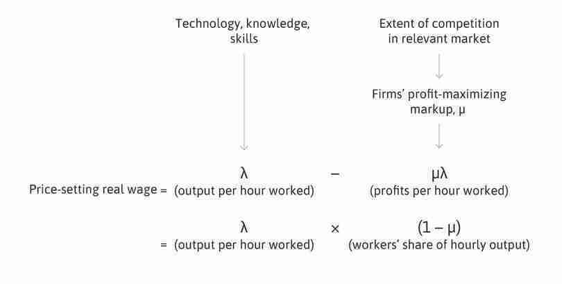
The price-setting real wage can be written as:
Using the numbers in our example, the price-setting real wage is:
The output per worker per hour (2 units) is split up as 1.5, which goes to the employees in the real wage, and 0.5 that goes to owners as profit. Owners get one-quarter of the output per worker and workers get three-quarters.
Hence:
This equation shows that, as a consequence of firms setting prices to get a markup, μ, the output produced per worker in the economy is divided into the share that goes to workers as wages (1 − μ) and the share that goes to owners as profits (μ).
Price-setting and the price-setting real wage, in diagrams
In Figure 8.5, we showed how to derive the economy-wide wage-setting curve from the game between the worker and the employer, when we vary the economy-wide unemployment rate.
In this section, we do the parallel analysis to derive the economy-wide price-setting curve from the price-setting firm’s profit-maximizing behaviour, when we vary the economy-wide demand for output.
For the simple model, we continue to assume that there is just a single firm in the economy with labour as its only input.
We now show how to derive the price-setting curve diagrammatically using the same numerical example.
Figure 8.10 shows how the inputs (nominal wage, unit cost, markup) and outputs (price and quantity) of the firm’s profit-maximization problem are illustrated in the diagram.
Next, we show in a diagram with employment on the horizontal axis and the real wage on the vertical axis, the combination of real wage and employment associated with point A in Figure 8.10. To translate the quantity produced (60 million) into the number of workers employed, we assume a working day of 7 hours. So in a day, given the per-hour productivity we have assumed (2 units per worker per hour shown in the dashed line in the lower panel of Figure 8.11), each worker produces 14 units. To produce 60 million units, 4.3 million workers are needed. This is shown on the horizontal axis of the lower panel.
The price-setting real wage at point A is 1.5 as we calculated above, and is shown in the lower panel. A characteristic of this model is that whatever the level of output and employment, the profit margin is 0.5. This implies that the price-determined real wage does not vary with employment and we therefore label the horizontal line at W/P = 1.5 in the lower panel of Figure 8.11 the price-setting real wage (the price-setting curve). We work out an example to illustrate this.
Different points on the price-setting (PS) curve: Effects of an increase in economy-wide demand for goods and services
Figure 8.12 shows the outcome for the real wage of the price-setting decisions of firms when there is an increase in economy-wide demand for goods and services. To make the example as simple as possible, we continue to assume there is a single firm in the economy. However, the lessons of this model can be applied to the real-world case where there are large numbers of firms, each of which faces a downward-sloping demand curve for its differentiated product. Then, instead of a single price, P, as the denominator in the real wage, W/P, each firm will set its price using the same method to maximize its profits. But the overall price level in the economy will be the outcome of the decisions by all firms.
An increase in demand for goods and services in the economy shifts the demand curve to the right. We assume that demand increases by a constant factor at every price. This means that the demand curve rotates around the point where it intercepts the vertical axis (as shown in Figure 8.12). When the demand curve shifts like this, there is no change in the markup at the given price. So this means that the firm will be setting the same profit-maximizing price whenever the demand curve shifts in this way.
In the example, the demand curve shifts by a factor of 1.05. This means that at the given price, the quantity is 5% higher. So the quantity produced rises by 5%, from 60 to 63 million units.
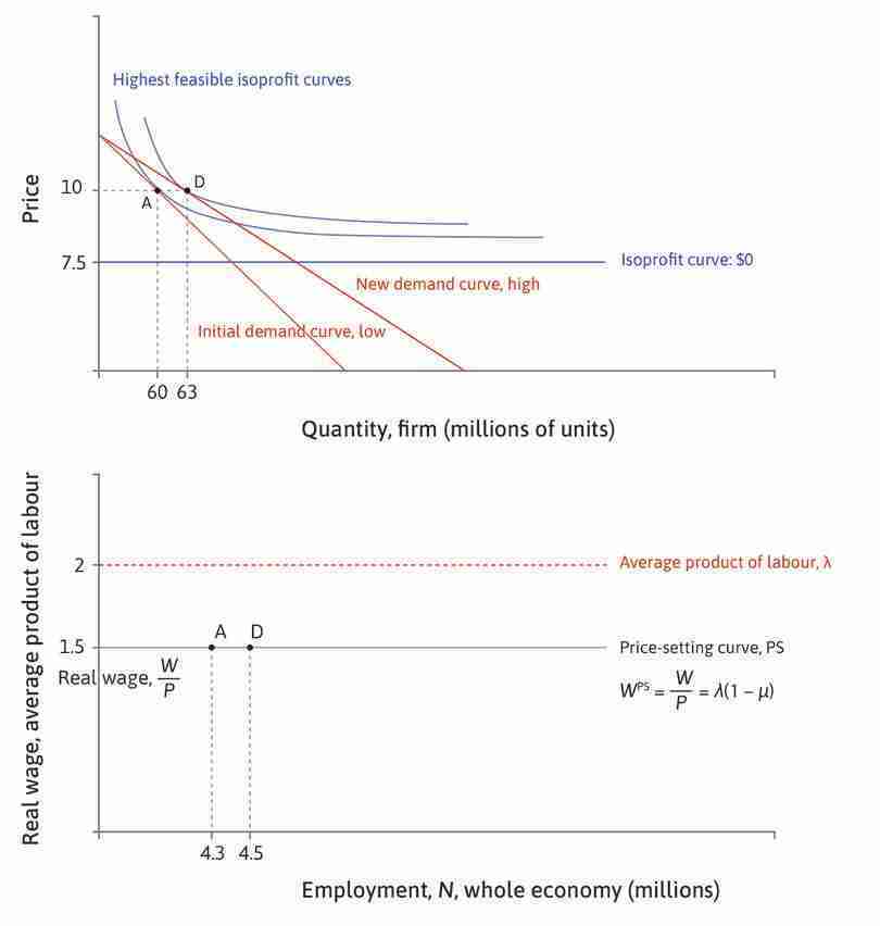
The price-setting curve: The effect of an increase in economy-wide demand for goods and services.
Figure 8.12 The price-setting curve: The effect of an increase in economy-wide demand for goods and services.
The new profit-maximizing outcome is at point D in Figure 8.12. Employment has also risen by 5% from 4.3 to 4.5 million workers.
By varying economy-wide demand we can derive more points like A and D, and so confirm that the price-setting real wage curve is a horizontal line.
So what we call the price-setting ‘curve’ is not really much of a curve—it is just a single number that gives the value of the real wage that is consistent with the markup, when all firms set their price to maximize their profits. In our numerical example, this number is 1.5.
To sum up, using our assumptions that neither productivity nor the markup vary with the level of employment, the value of the price-setting real wage is constant and is therefore shown, as in Figure 8.12, as a horizontal line.
What shifts the price-setting curve up or down?
Both from the diagram and the equation, we can see that the price-setting real wage will increase if productivity increases or if the markup falls. But what mechanisms bring this about?
Higher labour productivity
Returning to our example, if productivity doubles from 2 to 4 units produced per hour, then:
So the price-setting real wage doubles from 1.5 to 3.
- nominal wage
- The actual amount received in payment for work, in a particular currency. Also known as: money wage. See also: real wage.
Digging a bit deeper, we can see that the increase in productivity has halved the firm’s marginal cost (to $3.75). To keep its markup unchanged at 25% (since competitive conditions are assumed to be unchanged), the firm reduces its price to $5—it halves its price. The nominal wage is unchanged at $15 per hour, so the real wage has doubled to 3.
The mechanism by which higher productivity raises the price-setting real wage is summarized as follows. Higher productivity reduces costs and firms cut their prices. The result is a higher real wage.
More competition resulting in a lower markup
The price-setting real wage will increase if the demand curve becomes more elastic, that is if the markup in the economy falls as a result of more intense competition. This makes sense because, with fiercer competition, the share of profits will be lower and real wages will rise.
Suppose the markup falls from 0.25 to 0.2. Then:
In words, the real wage rises from 1.5 to 1.6.
The mechanism by which a lower markup raises the price-setting real wage is as follows—a lower markup reduces the price the firm can set because of the more intense competition. The result is a higher real wage.
What if the nominal wage rises?
What happens to the price-setting real wage if the nominal wage increases? Suppose the hourly wage increases from $15 to $16. This increases the marginal cost from $7.50 to $8.00. Hence:
So the real wage is:
The answer is that nothing happens to the real wage on the price-setting curve when the nominal wage increases. The reason is that, to maximize their profits, firms raise their prices to keep the markup (the profit margin divided by the price) unchanged, which means that prices increase by the same proportionate amount as wages.
Summary
We now summarize what determines the height of the price-setting curve. Later in the unit, we will look at how government policy can affect this.
- Labour productivity: For any given markup, the level of labour productivity—how much a worker produces in an hour—determines the real wage on the price-setting curve. The greater the level of labour productivity (or equivalently, the average product of labour, called lambda, λ), the higher the real wage that is consistent with a given markup. In Figure 8.12, higher labour productivity shifts the dashed line upwards, and, keeping the markup unchanged, the price-setting curve will shift upwards, raising the real wage.
Higher productivity pushes the price-setting curve upwards. Shares stay the same; the price-setting real wage is higher.
- Competition: You know from the previous unit that the intensity of competition facing firms determines the extent to which they can profit by charging a price that exceeds their costs, that is, their markup. The more intense the competition, the lower the markup. Since this leads to lower prices across the whole economy, it implies higher real wages, pushing the price-setting curve upwards.
More competition in markets for goods and services pushes the price-setting curve upwards. Workers get a bigger share; the price-setting real wage is higher.
We summarize the influences on the price-setting curve in Figure 8.13.
Determinants of the price-setting curve.
Figure 8.13 Determinants of the price-setting curve.
- price elasticity of demand
- The percentage change in demand that would occur in response to a 1% increase in price. We express this as a positive number. Demand is elastic if this is greater than 1, and inelastic if less than 1.
Find out more The size of the markup chosen by the firm
We can find a formula that shows that the markup is high when the elasticity of demand is low.
The firm maximizes its profits by setting its price where the slope of the isoprofit curve is equal to the slope of the demand curve, and we know that the slope of the demand curve is related to the price elasticity of demand:
Rearranging this formula:
We also know from Section 7.5:
When the two slopes are equal:
Rearranging this gives us:
The left-hand side is the profit margin as a proportion of the price, which is called the markup. Therefore:
The firm’s markup is inversely proportional to the elasticity of demand.
Hence:
In the example, if μ = 0.25 (the elasticity is 4) and MC = $7.50, then we can calculate the price:
Question 8.3 Choose the correct answer(s)
Suppose the nominal wage W = $10, the markup μ = 0.5, and the marginal cost is $5. Based on this information and the discussion in this section, which of the following statements are true?
- The elasticity of demand is the inverse of the markup, so is 1 / 0.5 = 2.
- The marginal cost is equal to half of the price (MC = (1 − 0.5)P).
- The price P is $10 and so is the nominal wage, so the real wage is 1.
- The real wage is equal to λ(1 − μ), which means 1 = λ(1 − 0.5), so λ is 2.
Question 8.4 Choose the correct answer(s)
Suppose the nominal wage W = $20, the markup μ = 0.4, the marginal cost is $15, and the firm’s profit-maximising quantity is Q = 50. Assume there are no fixed costs. Based on this information and the discussion in this section, which of the following statements are true?
- The price P is $25, so the real wage W/P is 0.8.
- The price P is $25, so the firm’s profits are (P − MC) × Q = (25 − 15) × 50 = $500. (Q, P) = (100, 20) also gives a profit of $500.
- Average productivity (λ) is 4/3 (= 1.33).
- μ is 0.4 and λ is 4/3, so μλ = 0.4 × 4/3 = 8/15.
8.6 Wages, profits, and unemployment in the aggregate economy
Putting the wage-setting and the price-setting curves together, we have a model for the macroeconomy from which we can directly determine the real wage and the level of structural employment.
- Nash equilibrium
- A set of strategies, one for each player in the game, such that each player’s strategy is a best response to the strategies chosen by everyone else.
We ask what the equilibrium of an economy will be, as depicted by the two curves. Remember, a Nash equilibrium is a situation in which none of the actors would like to change what they are doing, given what the others are doing.
Who are the actors? Recall that the firm has two departments: Marketing and human resources (HR), both of course operating under the direction of the owners of the firm or their top managers. HR knows, for any level of unemployment, the real wage that is the least cost way to get workers to work. Marketing knows, given the demand curve facing the firm, what the price of the goods sold should be to maximize the firm’s profits.
When we say that in the Nash equilibrium, ‘none of the actors would like to change what they are doing, given what the others are doing’, we are referring to the actions taken by Marketing and HR in respectively setting the price and the nominal wage.
Their interaction is summarized in Figure 8.14.
| Department | … knows | … and on this basis sets the firm’s |
|---|---|---|
| HR | Prices and wages in other firms, and the unemployment rate in the economy | Nominal wage, W |
| Marketing | All of the above, and firm’s demand function | Price of output, P |
The two departments in each firm determine the wage and price set by the firm.
Figure 8.14 The two departments in each firm determine the wage and price set by the firm.
Can anybody do better? Is the intersection of the two curves a Nash equilibrium?
To determine the equilibrium of this economy, we need to ask the question: ‘Can anybody do better?’ In the left-hand panel of Figure 8.15, we ask if HR can do better. We see that, for any combination of wage and employment below the wage-setting curve, they are sounding the alarm—nobody is working, we need to raise wages. Above the wage-setting curve, they are sounding a different alarm—the firm is throwing away money by paying too much.
In the right-hand panel, we ask if Marketing can do better. We see that, for any combination of wage and employment above the price-setting wage, the firm can charge a higher price and make more profits. Below the price-setting curve, the marketing department is alarmed because the firm is losing customers and should lower the price.
The Nash equilibrium of the economy
By superimposing the wage-setting curve on the price-setting curve in the right-hand panel of Figure 8.15, we have a picture of the macroeconomy, illustrated in Figure 8.16.
- incentive
- Economic reward or punishment, which influences the benefits and costs of alternative courses of action.
- equilibrium unemployment
- The number of people seeking work but without jobs, which is determined by the intersection of the wage-setting and price-setting curves. This is the Nash equilibrium of the labour market and product market where neither employers nor workers could do better by changing their behaviour. See also: involuntary unemployment, structural unemployment, wage-setting curve, price-setting curve, WS/PS model, inflation-stabilizing rate of unemployment.
- involuntary unemployment
- A person who is seeking work, and willing to accept a job at the going wage for people of their level of skill and experience, but unable to secure employment is involuntarily employed.
- structural unemployment
- The level of unemployment at the Nash equilibrium of the labour and product market model.
The equilibrium of the economy is the point at which the wage- and price-setting curves intersect, shown by X in the figure.
- Workers are working: They have no incentive to shirk. If they demanded higher pay, their employer would refuse, or replace them.
- HR does not want to change the wage: The workers are motivated, at the lowest possible cost.
- Marketing is satisfied: Prices have been set at the profit-maximizing level.
What about the unemployed, who, apart from not having a job, are identical to the employed? They are surely unhappy in this situation. Those who fail to get jobs would rather have a job, but in this situation there is no way for them to get one—not even if they offer to work at a lower wage than others. The unemployment at the equilibrium of the labour and product market in the economy—equilibrium unemployment—is involuntary unemployment; also known as structural unemployment.
This is a Nash equilibrium because all parties are doing the best they can (even the unfortunate unemployed), given what everyone else is doing.
Question 8.5 Choose the correct answer(s)
Which of the following statements about outcome X in Figure 8.16 are correct?
- At X, employees are on their best response function for effort. This means that putting effort in is their best strategy. A positive employment rent ensures this.
- X is on the wage-setting curve, which is determined by the point of tangency between a firm’s isocost and the workers’ best response function curve for effort.
- The employers know that once the unemployed get jobs at a lower wage, they will shirk. Therefore, the unemployed will not be offered a job at a lower wage.
- Above the price-setting curve, the markup is too low, so the firm can increase profits by raising prices.
Question 8.6 Choose the correct answer(s)
Figure 8.16 depicts the model of the aggregate economy. Consider a reduction in the degree of competition faced by the firms. Which of the following statements regarding the effects of reduced competition are correct?
- Decreased competition implies a higher markup. This decreases the share of output claimed by the workers, reducing their real wage. Hence, the price-setting curve shifts downwards.
- The wage-setting curve is determined by the supply of labour. Therefore, it is unaffected.
- Decreased competition leads to a lower price-setting curve, while the wage-setting curve is unaffected. Therefore, the equilibrium (the intersection of the two curves) shifts downwards and to the left, implying lower real wage and higher unemployment.
- With the price-setting curve shifting downwards, the intersection of the two curves moves down the wage-setting curve to where there is higher unemployment.
8.7 Unemployment as a characteristic of equilibrium
We now show why there will always be structural unemployment in the equilibrium of the aggregate economy.
- excess supply
- A situation in which the quantity of a good supplied is greater than the quantity demanded at the current price. See also: excess demand.
- substitution effect
- The effect for example, on the choice of consumption of a good that is only due to changes in the price or opportunity cost, given the new level of utility.
- income effect
- The effect, for example, on the choice of consumption of a good that a change in income would have if there were no change in the price or opportunity cost.
Unemployment means that there are people seeking work but not finding it. This is also called excess supply in the labour market, meaning that demand for labour at the given wage is lower than the number of workers willing to work for that wage. Those unable to get a job are involuntarily unemployed. To understand why there will always be unemployment in equilibrium (where the wage- and price-setting curves intersect), we contrast the wage-setting curve with the labour supply curve. We shall see that the wage-setting curve is always to the left of the labour supply curve: for any real wage, the gap between the level of employment on the wage curve and on the labour supply curve measures involuntary unemployment.
In our model, we assume that higher wages do not—in the economy as a whole—lead more people to offer more hours at work. At higher wages some people seek (and find) more hours of work, and others seek (and find) shorter hours. The first is the substitution effect of a wage increase, and the second is the income effect. We introduced these effects in Section 4.9. For simplicity, we draw a vertical labour supply curve such that these two effects cancel out. But this is not important. The model would not be different if higher wages led to either more or fewer people seeking work. To see this, you can experiment with labour supply curves with different shapes in Figure 8.16.
Why will there always be some involuntary unemployment in equilibrium?
- If there was no unemployment: The cost of job loss would be zero (no employment rent) because a worker who loses her job can immediately get another one at the same pay.
- Therefore, some unemployment is necessary: It means the employer can motivate workers to provide effort on the job, which is essential to production.
- Therefore, the wage-setting curve is always to the left of the labour supply curve.
- It follows that in any equilibrium, where the wage- and price-setting curves intersect, there must be unemployed people.
Exercise 8.3 Is this really a Nash equilibrium?
In this model, the unemployed are no different from the employed (except for their bad luck). Imagine you are an employer, and one of the unemployed comes to you and promises to work at the same effort level as your current workers, but for a slightly lower wage.
- How would you reply?
- Does your reply help explain why unemployment must exist in a Nash equilibrium?
Question 8.7 Choose the correct answer(s)
Suppose the real wage increases. Which of the following statements about the labour supply of a worker are correct?
- As the real wage rises, the worker feels richer. This would induce him to work less, that is the income effect is negative.
- The real wage is the price of consuming leisure. Therefore, when the wage rises, free time becomes more expensive relative to consumption goods (which are purchased using the wage income). Hence, the worker would substitute out of consuming leisure into consuming goods, implying lower free time and higher labour supply.
- The income and substitution effects always work against each other, leading to higher labour supply at lower wages, and lower labour supply at higher wages.
- The negative income effect and the positive substitution effect always work against each other. At high wages, the former more than offsets the latter, implying that the worker reduces his labour supply (he already earns enough).
8.8 Why was unemployment higher in Spain than in Germany?
Recall that at the beginning of this unit we contrasted the unemployment rates of Germany and Spain. Figure 8.17 provides more details, comparing unemployment in Germany and Spain from 1960 to 2018. We can use the WS/PS model developed in this unit to propose some explanations for the wide gap between the unemployment rates in these two large European countries.
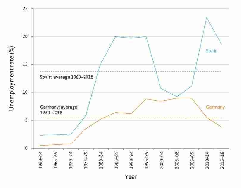
Unemployment in Spain and Germany (1960–2018).
Figure 8.17 Unemployment in Spain and Germany (1960–2018).
Data from 1960–2004: David R. Howell, Dean Baker, Andrew Glyn, and John Schmitt. 2007. ‘Are Protective Labor Market Institutions at the Root of Unemployment? A Critical Review of the Evidence’. Capitalism and Society 2 (1) (January). Data from 2005 to 2018: OECD. 2019. OECD Statistics.
The model directs our attentions to the position of the wage- and price-setting curves. The point at which they cross pins down unemployment at the Nash equilibrium. The differences in the average unemployment rates over many decades between Germany and Spain suggests that structural unemployment in the two countries must be different.
The table in Figure 8.18 brings together summary data that helps to explain the Germany–Spain comparison.
| Unemployment rate (%) | Generosity of unemployment benefits (%) | Openness of the economy to global competition (% of GDP) | Labour productivity in manufacturing (2005 US$) | |
|---|---|---|---|---|
| Germany | 6.8 | 26.9 | 71.0 | 43.3 |
| Spain | 15.4 | 31.9 | 65.1 | 30.6 |
Determinants of structural unemployment in Spain and Germany (1976–2011).
Figure 8.18 Determinants of structural unemployment in Spain and Germany (1976–2011).
Data from 1976–2004: David R. Howell, Dean Baker, Andrew Glyn, and John Schmitt. 2007. ‘Are Protective Labor Market Institutions at the Root of Unemployment? A Critical Review of the Evidence’. Capitalism and Society 2 (1) (January). Data from 2005 to 2011: OECD. 2015. OECD Statistics.
Note: Generosity of unemployment benefits is measured as Gross Unemployment Benefit Replacement Rates. Openness of the economy to global competition is exports plus imports as a share of GDP. Labour productivity is gross value added per hour worked, in manufacturing sector, measured in 2005 US$. All data is averaged over the period 1976–2011.
In the model, the structural unemployment rate (unemployment at the Nash equilibrium) is increased by factors that shift the wage-setting curve upwards and reduced by factors that shift the price-setting curve downwards.
Comparing these two countries, we can see that Spain has a more generous unemployment benefit regime. Ceteris paribus, the higher unemployment benefits in Spain shift the wage-setting curve upwards relative to the case of Germany.
We shall see the importance of the ceteris paribus assumption later in this unit. There are countries with more generous unemployment benefits than Spain with much lower structural unemployment. In those countries, generous unemployment benefits were not simply generous but were designed to help the unemployed re-enter employment quickly. This was not the case in Spain.
Turning to the price-setting curve, from the model we know that, if there is stronger competitive pressure on firms, the price-setting curve will shift upwards. In Figure 8.18, using data from 1976 to 2011, we use the measure of the openness of the economy to international trade, calculated as the sum of its exports plus its imports divided by GDP as a proxy for the pressure of competition. According to this indicator, the German economy is much more open to competition than is the Spanish economy. Ceteris paribus, this shifts the price-setting curve upwards in Germany relative to Spain.
The data in the final column of the table highlights the difference in output per worker hour between the two economies. The measure we use is hourly productivity in manufacturing because it is likely that productivity is better measured there than elsewhere in the economy. By this measure, productivity in Germany is 60% higher than in Spain. Ceteris paribus, this shifts the price-setting curve upwards in Germany relative to that in Spain.
Figure 8.19 illustrates how these differences can be shown in the model. Spain’s structural unemployment at point X is higher than Germany’s at Y, as a result of a higher wage-setting and a lower price-setting curve. The model predicts that Germany’s real wage is higher than Spain’s.
8.9 Declining competition and increasing inequality in the US
Firms have become more powerful in relation to their customers since the 1980s. And we shall use the model of the labour market and product market to see how this phenomenon increases economic inequality. A fall in the degree of competition in markets for goods and services, ceteris paribus, entails higher structural unemployment and a higher share of profits. Both raise inequality among households.
Recent research shows the rise in the markup in the US, and in many other countries. Figure 8.20 for the US, shows a falling average markup from the mid-1960s to 1980, a rapid increase until 2000, and then, after a decade of stability, a renewed rise since the global financial crisis. The average markup is more than twice now what it was in 1980.
The estimated average markup for firms in the US (1955–2016).
Figure 8.20 The estimated average markup for firms in the US (1955–2016).
Jan De Loecker, Jan Eeckhout, and Gabriel Unger. 2018. The Rise of Market Power and the Macroeconomic Implications. NBER Working Paper.
Note: Our measure of the markup is 1 minus the inverse of the measure used in the source data.
- economic profit
- A firm’s revenue minus its total costs (including the opportunity cost of capital).
Over the same period, the share of the economy’s income going in economic profits to the owners of firms has been increasing, as illustrated also for the US in Figure 8.21.
The share of economic profits in income in the US (1984–2014).
Figure 8.21 The share of economic profits in income in the US (1984–2014).
Simcha Barkai 2016. Declining Labor and Capital Shares. Stigler Center for the Study of the Economy and the State, New Working Paper Series No. 2.
Note: In estimating the profit share for the US economy the author divides income into three parts. One is the labour share. The rest is ‘profits’, which are split into the other two shares. The ‘capital share is the opportunity cost of capital as a share of income; the remainder is what is labelled in the chart ‘Profit share’ and is the share of economic profits in income.
Listen to John Van Reenen, an economist, talking about the rise of superstar firms and the challenges they pose for policymakers seeking to sustain or restore a competitive economy.
The research on trends in both markups and the share of profits points to the central role of declining competition in markets for goods and services. This development suggests that there has been a long-term shift in the balance of power in the US economy (and in some other countries) toward the owners of firms and away from their customers.
Figure 8.22 shows the increase in inequality among US households in their market income (before the payment of taxes and receipt of transfers) from 1970 to 2015.
The Gini coefficient for market income in the US (1970-2015).
Figure 8.22 The Gini coefficient for market income in the US (1970-2015).
Anthony Atkinson, Joe Hasell, Salvatore Morelli, and Max Roser. 2017. The Chartbook of Economic Inequality.
The upward trend in inequality among US households from 1980 measured by the Gini coefficient is clear. As we shall see in the next section, the model of the labour and product market predicts that a decline in competition in product markets leads to a rise in inequality measured by the Gini coefficient. We return in Section 8.12 to US economic performance.
8.10 The labour and product market model and inequality: Using the Lorenz curve and Gini coefficient
- Lorenz curve
- A graphical representation of inequality of some quantity such as wealth or income. Individuals are arranged in ascending order by how much of this quantity they have, and the cumulative share of the total is then plotted against the cumulative share of the population. For complete equality of income, for example, it would be a straight line with a slope of one. The extent to which the curve falls below this perfect equality line is a measure of inequality. See also: Gini coefficient.
- Gini coefficient
- A measure of inequality of any quantity such as income or wealth, varying from a value of zero (if there is no inequality) to one (if a single individual receives all of it).
As we have seen, the model for the aggregate economy determines not only the level of employment, unemployment, and the wage rate, but also the division of the economy’s output between workers (both employed and unemployed) and employers. It is therefore also a model of the distribution of income in a simple economy in which labour is the only input and there are just these two classes. The classes are employers—who are the owners of the firms—and workers—some of whom are without work.
The distribution of income at the Nash equilibrium
As we did in Unit 5, we can construct the Lorenz curve and calculate the Gini coefficient for the economy in this model. Refer back to Unit 5 to recall how to construct the Lorenz curve and calculate the Gini coefficient.
In the left-hand panel of Figure 8.23, we show an economy with 80 identical employees of 10 identical firms. As you can see, there are 10 unemployed people. Each firm has a single owner. The economy is in equilibrium at point A, at which the real wage is both sufficient to motivate workers to work and consistent with the firm’s profit-maximizing price markup over costs.
The right-hand panel shows the Lorenz curve for income in this economy. Because there are no unemployment benefits, the unemployed people receive no income, the Lorenz curve (the solid blue line) begins on the horizontal axis to the right of the left-hand corner. The price-setting curve in the left-hand panel indicates that total output is divided up so that workers receive a 60% share and their employers receive the rest. In the right-hand panel, this is shown by the second ‘kink’ in the Lorenz curve, where we see that the poorest 90 people in the population (the 10 unemployed workers and the 80 employees, shown on the horizontal axis) receive 60% of the total output (on the vertical axis). The size of the shaded area measures the extent of inequality, and the Gini coefficient is 0.36.
The Lorenz curve is made up of three line segments, with the beginning point having coordinates of (0, 0) and the endpoint (1, 1). The first kink in the curve occurs when we have counted all the unemployed people.
The second is the interior point, whose coordinates are (fraction of total number of economically active population, fraction of total output received in wages). The fraction of output received in wages, called the wage share in total income, s, is:
When does inequality increase?
The shaded area in the figure—and hence inequality measured by the Gini coefficient—will increase if:
- A larger fraction of the employees is without work (higher unemployment rate): The first kink shifts to the right.
- The real wage falls (or equivalently, the markup rises) and nothing else changes: The second kink shifts downwards.
- Productivity rises and nothing else changes (real wages do not rise): This implies that the markup rises, so again the second kink shifts downwards.
More competition in markets for goods and services, lower inequality
What can change the level of employment and the distribution of income between profits and wages in equilibrium? Follow the analysis in Figure 8.24 to see what would happen if there were an increase in the degree of competition faced by firms, perhaps as a result of a fall in the barriers preventing firms from other countries competing in this economy’s markets.
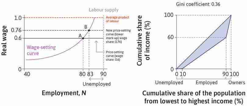
The effect of an increase in the extent of competition faced by firms: The price-setting curve shifts upwards and inequality falls.
Figure 8.24 The effect of an increase in the extent of competition faced by firms: The price-setting curve shifts upwards and inequality falls.
The initial equilibrium
We start from the equilibrium at A with a Gini coefficient of 0.36. Suppose that the degree of competition faced by firms is increased.
Figure 8.24a We start from the equilibrium at A with a Gini coefficient of 0.36. Suppose that the degree of competition faced by firms is increased.
A new equilibrium
The markup charged by firms in the market will decrease, and so the price-setting curve will be higher. The new equilibrium is at B.
Figure 8.24b The markup charged by firms in the market will decrease, and so the price-setting curve will be higher. The new equilibrium is at B.
A new, lower Gini coefficient
At the new equilibrium there is a higher wage and a higher level of employment. Stronger competition means that firms have weaker market power—the share going to profits falls, and the share going to wages rises. Inequality falls: the new Gini coefficient is 0.19.
Figure 8.24c At the new equilibrium there is a higher wage and a higher level of employment. Stronger competition means that firms have weaker market power—the share going to profits falls, and the share going to wages rises. Inequality falls: the new Gini coefficient is 0.19.
The markup would decrease, and as a result the real wage shown by the price-setting curve would increase, leading to a new equilibrium at point B with a higher wage and a higher level of employment. The share of output going to profits falls, and the share going to wages rises—inequality falls.
Question 8.8 Choose the correct answer(s)
Figure 8.23 is the Lorenz curve associated with a particular labour market equilibrium. In a population of 100, there are 10 firms, each with a single owner, 80 employed workers, and 10 unemployed workers. The employed workers receive 60% of the total income as wages. The Gini coefficient is 0.36. In which of the following cases would the Gini coefficient increase, keeping all other factors unchanged?
- A rise in the unemployment rate would shift the first kink of the Lorenz curve to the right. This shifts the curve downwards, increasing the Gini coefficient.
- A rise in the real wage would raise the second kink of the Lorenz curve. This shifts the curve upwards, decreasing the Gini coefficient.
- This implies a rise in the markup, or equivalently, a fall in the wage share in total income. This shifts the second kink of the Lorenz curve downwards, increasing the Gini coefficient.
- A rise in the degree of competition would raise the price-setting curve in the model of the labour market, resulting in higher employment and higher wage share. This shifts the first kink of the Lorenz curve to the left and the second kink upwards, reducing the Gini coefficient.
8.11 Labour unions: Bargained wages and the union voice effect
- trade union
- An organization consisting predominantly of employees, the principal activities of which include the negotiation of rates of pay and conditions of employment for its members.
The model of the aggregate economy presented so far is about firms and individual workers. But, in many countries, labour unions play a big part in how the labour market works.1 A trade union (or labour union) is an organization that can represent the interests of a group of workers in negotiations with employers over issues such as pay, working conditions, and working hours. The resulting contract is between the firm or organization representing employers and the labour union.2
As you can see from Figure 8.25, the fraction of the workforce employed under collective bargaining agreements negotiated by labour unions varies greatly between countries, from virtually all workers in France and some northern European economies, to hardly any in the US and South Korea.
Share of employees whose wages are covered by collective bargaining agreements (early 2010s).
Figure 8.25 Share of employees whose wages are covered by collective bargaining agreements (early 2010s).
Jelle Visser. 2015. ‘ICTWSS Data base. version 5.0’. Amsterdam: Amsterdam Institute for Advanced Labour Studies AIAS. Updated October 2015.
Labour unions and the bargained wage-setting curve
Where workers are organized into trade unions, the wage is not set by the HR department but instead is determined through a process of negotiation between a union representing workers and the firm’s HR department. Although the wage must always be at least as high as the wage indicated by the wage-setting curve for the given level of unemployment, the bargained wage can be above the wage-setting curve.
The threat of going on strike
The reason is that the employer’s threat to dismiss the worker is now not the only exercise of power that is possible. The union can threaten to ‘dismiss’ the employer (at least temporarily) by going on strike, that is, withdrawing the employees’ labour from the firm.
Therefore, the firm must agree to a wage that ensures that it will have the required work done to produce the goods or services on which its profits depend. This requires both that:
- The workers will provide sufficient effort when they come to work: The wage-setting curve determines this.
- The workers will come to work rather than go on strike: A bargained wage-setting curve will determine this.
We can think of a ‘bargaining curve’ lying above the wage-setting curve, which indicates the wage that the union–employer bargaining process will produce for every level of employment.
The relative bargaining power of the union and the employer determines how far this bargaining curve lies above the wage-setting curve. The union’s power depends on the ability to withhold labour from the firm, so its bargaining strength will be greater if it can ensure that during a strike, no other workers will offer their services to the firm.
This and the other determinants of bargaining power depend on the laws and social norms in force in an economy. In many countries, for example, it is a serious violation of a social norm among workers to seek employment in a firm whose workers are on strike.
To see the difference that a labour union can make, let’s see how the labour market would work if, instead of the employer setting the wage and the employees individually responding, the process would now be as shown in Figure 8.26.
| The union sets the wage | ⇨ | The employer informs workers that insufficient work will result in job termination | ⇨ | Employees respond to the wage and the prospect of dismissal by choosing how hard to work |
If the union sets the wage.
Figure 8.26 If the union sets the wage.
In this case, the employer no longer sets the wage that maximizes profits (the point of tangency of the isocost line for effort and the best response curve at point A in Figure 8.27). Use the analysis in Figure 8.27 to see what happens when the union, rather than the firm, sets the wage. To see the outcome for structural unemployment in the economy, see Figure 8.28.
If the union sets the firm’s wage instead of the employer.
Figure 8.27 If the union sets the firm’s wage instead of the employer.
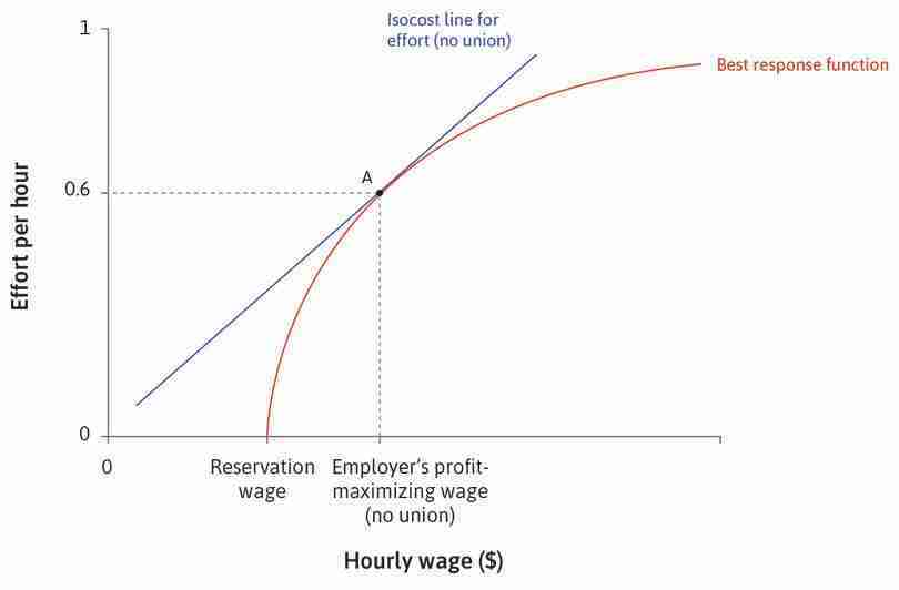
The employer sets the wage
At point A, the employer sets the wage that maximizes profits at the point of tangency of the isocost line and the best response function.
Figure 8.27a At point A, the employer sets the wage that maximizes profits at the point of tangency of the isocost line and the best response function.
As shown in Figure 8.27, the wage will be higher than that preferred by the employer. Workers will now be working harder, but wages increase by more than productivity, so firms receive less effort for each dollar spent on wages. It follows that profits will be lower than without the union, that is, on the flatter isocost line passing through C.
By translating Figure 8.27 to the model of the labour market and product market in Figure 8.28, we see that the bargained wage-setting curve lies above the wage-setting curve. Looking at the equilibrium where the bargained wage-setting curve intersects with the price-setting curve, the wage is unaffected, but the level of employment is lower.
Unions in the model and in the data
Paradoxically, it seems from the model that the union’s success in bargaining would harm workers, since the real wage is unchanged and more people are out of work. But if we look at the data on union bargaining coverage and unemployment in Figure 8.29, unemployment does not seem to be higher in countries where union bargains are important in wage-setting.
Austria, with almost all employees covered by union wage bargains, has a lower unemployment rate (averaged over 2000–2014) than the US, where fewer than one in five workers is covered by union contracts. Spain and Poland both had massive unemployment over this period, but union coverage was very high in Spain and very low in Poland.
Collective wage bargaining coverage and unemployment across the OECD.
Figure 8.29 Collective wage bargaining coverage and unemployment across the OECD.
Jelle Visser. 2015. ‘ICTWSS Data base. version 5.0’. Amsterdam: Amsterdam Institute for Advanced Labour Studies AIAS. Updated October 2015.
Therefore, the fact that unions can push the wage-setting curve upwards to the new ‘bargained wage-setting curve’ must not be the entire story.
A powerful union may choose restraint
One possible explanation is that a powerful union may choose not to raise the wage, even if it has the power to do so. This is because even a very powerful union can only set the wage, and it cannot determine how many people the firm hires. Too high a wage may squeeze profits sufficiently to lead the firm to close down or cut back on employment.
Unions may choose to restrain their use of bargaining power. If their wage-setting covers a substantial part of the economy, they will take into account the effect of their wage decision on the wages and employment of workers in the economy as a whole.
The union voice effect
Unions differ in other ways.
Suppose that, over time, the employer and the trade union develop a constructive working relationship—for example, solving problems that arise in ways that benefit both employees and the owners. The employees may interpret the employer’s recognition of the trade union, and its willingness to compromise over a higher wage, as a sign of goodwill.
As a result, the employees might identify more strongly with their firm and experience effort as less of a burden than before, shifting their best response curve upwards in Figure 8.30.
The result of the greater bargaining power of the workers, and their reciprocation of the company’s worker-friendly policy, is shown as point D in the Figure 8.30. The wage is the same as in the previous case but, because worker effort is higher, the firm’s profits are higher. Note that in the example shown, the firm is still worse off than it was in the absence of the union.
With the new best response function, there is of course an outcome for a wage-setting firm that is even better than D—where the isocost curve is tangent to it (not shown). However, this is not feasible. The workers will not exert the higher effort in the absence of the negotiations about wages and conditions opened up by the union’s role in wage-setting.
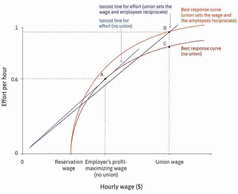
The union sets the firm’s wage, and employees reciprocate.
Figure 8.30 The union sets the firm’s wage, and employees reciprocate.
The employer sets the wage
At point A, the employer sets the wage that maximizes profits at the point of tangency of the isocost line and the best response curve.
Figure 8.30a At point A, the employer sets the wage that maximizes profits at the point of tangency of the isocost line and the best response curve.
The employer recognizes a trade union
If the employees interpret the employer’s recognition of the trade union, and its willingness to compromise over a higher wage, as a sign of goodwill, the best response curve shifts upwards.
Figure 8.30b If the employees interpret the employer’s recognition of the trade union, and its willingness to compromise over a higher wage, as a sign of goodwill, the best response curve shifts upwards.
The effect of a worker-friendly policy
The result of the greater bargaining power of the workers, and their reciprocation of the company’s worker-friendly policy, is shown as point D.
Figure 8.30c The result of the greater bargaining power of the workers, and their reciprocation of the company’s worker-friendly policy, is shown as point D.
Unions may raise or lower structural unemployment
We have shown two effects of the presence of a labour union, which we can now represent in the WS/PS diagram:
- The union forces the firm to pay a wage greater than the minimum necessary to induce the employees to work: The bargaining curve is always above the wage-setting curve.
- The union provides employees with a voice in how decisions are made: This may lower the disutility of effort and therefore reduce the lowest wage necessary to motivate employees to work effectively.
- union voice effect
- The positive effect on labour effort (and hence labour productivity) of trade union members’ sense that they have a say (a voice) in how the firm is run.
The two effects are illustrated in Figure 8.31. In this figure, we show the case in which the equilibrium level of employment is higher and unemployment lower with the union (point Y) than without (point X). This is because the second effect (called the union voice effect) that shifts the wage-setting curve downwards was greater than the bargaining effect that shifts the wage-setting curve upwards.
But it could have worked out the other way around. The bargained wage effect could have been greater than the union voice effect, in which case the effect of unions would have been to raise structural unemployment.
This provides a reason why the data in Figure 8.29 does not show any clear correlation (either positive or negative) between the extent of union contracts and the amount of unemployment.
Unions may also affect the average productivity of labour, which will shift the price-setting curve. If unions foster cooperation with management in solving production problems, the average product and the price-setting curve will rise (leading to higher wages and less unemployment). If unions resist productivity improvements, such as the introduction of new machinery or changes in work rules, then the effect will go in the opposite direction.
Question 8.9 Choose the correct answer(s)
Figure 8.27 depicts the effect of union wage-setting. What can we conclude from this figure?
- The isocost line is flatter through C than through A. This means that the firm receives less effort from workers for each dollar spent on wages. Therefore, the firm’s profit is lower at C.
- Due to the union effect, employees need to be paid a higher wage to work hard, compared to when there is no union. This shifts the wage-setting curve higher.
- If the employees reciprocate (for example, when they have a lower disutility of effort) and there is a ‘union voice effect’, this has an effect of shifting the wage-setting curve downwards. If this more than offsets the wage bargaining effect that shifts the wage-setting curve up, then there will be an overall decrease in unemployment.
- Unlike at A, at C the firm is not producing at the point of tangency between the isocost line and the best response curve. Therefore, it is no longer setting the profit-maximizing wage level.
Question 8.10 Choose the correct answer(s)
Which of the following statements regarding labour unions and wage bargaining are correct?
- The unions cannot determine how many people the firm hires.
- The unions would not ask for a wage lower than the firms’ profit-maximizing level. Therefore, the bargaining curve is always above the wage-setting curve.
- Demanding too high a wage may squeeze profits sufficiently, leading the firm to close down or cut back on employment. Therefore, unions may choose to restrain their bargaining power.
- Shutting down firms does not help the workers. The unions’ bargaining power comes from their threat to ‘dismiss’ the employer (at least temporarily) by going on strike (withdrawing the employees’ labour from the firm).
8.12 Rising markups and profit share, weaker trade unions, and rising inequality
The data on rising markups and profit share in the US since 1980 in Section 8.9 suggest that the extent of competition faced by firms has declined. In the WS/PS model, this is represented by a downward shift in the price-setting curve. The new equilibrium is at point B in Figure 8.32. The model predicts that a decline in the degree of competition and the resulting downward shift in the price-setting curve will bring about a rise in inequality for two reasons:
- A higher markup means a higher profit share: In the model with only labour costs, the markup is the profit share. See the new lower price-setting curve in Figure 8.32 and the fall in the wage share from 0.76 to 0.60.
- Unemployment in equilibrium is higher: In the figure for an economy of 100 people, the number of unemployed people rises from 7 to 10.
But the predicted rise in unemployment at point B did not occur in the US economy. That employment, if anything, rose, may be explained by the fact that trade unions became weaker in the US over this period in ways that shifted the wage-setting curve downward.
The union density rate, which measures the share of employees who belong to a union, fell from 20.1% in 1983 to 10.5% in 2018. As a result, it became easier (less costly) for employers to fire workers whose work they find unsatisfactory. This would increase the probability that a worker would be terminated if they were not working up to speed. From the previous section, this can be represented by a downward shift in the wage-setting curve (Figure 8.23). Over the same period, other changes in the labour market including the emergence of the gig economy, discussed in Section 6.14, have reduced the reservation wage of workers and contributed to the downward shift of the wage-setting curve.
Work through the analysis in Figure 8.32 to see how the combination of growing monopoly power, with a weaker bargaining position for workers, can realize the model’s prediction that inequality rises, without a rise in unemployment. Indeed, the example shown in the figure (point C) has lower unemployment than the initial situation at point A.
Rising monopoly power (the product market) and declining worker power (the labour market)—a new equilibrium.
Figure 8.32 Rising monopoly power (the product market) and declining worker power (the labour market)—a new equilibrium.
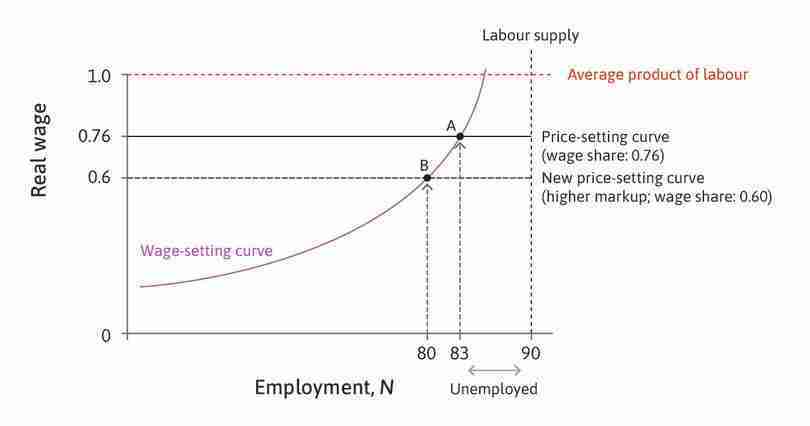
The new price-setting curve
Due to the decrease in the level of competition, the price-setting curve shifts down. The wage share falls to 0.6 and the unemployment rate increases to 10% (point B).
Figure 8.32b Due to the decrease in the level of competition, the price-setting curve shifts down. The wage share falls to 0.6 and the unemployment rate increases to 10% (point B).
The new wage-setting curve
Due to the weaker bargaining position of workers, the wage-setting curve also shifts down. Depending on how far the wage-setting curve shifts, unemployment can decrease compared to the initial situation, as shown by point C.
Figure 8.32c Due to the weaker bargaining position of workers, the wage-setting curve also shifts down. Depending on how far the wage-setting curve shifts, unemployment can decrease compared to the initial situation, as shown by point C.
Using Section 8.10, we can now illustrate the implications for inequality of the rise in monopoly power combined with the weakening of trade unions and emergence of the gig economy (Figure 8.33).
In this example, the impact of the rise in the profit share in pushing the Lorenz curve away from the line of equality outweighs the impact of the fall in unemployment in reducing inequality.
The combination of the model (Figures 8.32 and 8.33), with the data on markups, and the profit share in Figures 8.20 and 8.21 in Section 8.8, support the hypothesis that falling competition in markets for goods and services in the US is part of the reason for rising inequality among households, as shown by the Gini coefficient in Figure 8.22. The trends in these charts are similar, but other factors may still be at work.
Two other important factors affecting the inequality of household market incomes are automation and the China shock. People in particular occupations have been the losers from the development of new technologies that replace routine work. Other losers have been those working in particular industries subject to competition from imports from China, as it rapidly industrialized and became a large supplier of manufactured goods, such as furniture and toys.
8.13 Labour market policies to address unemployment and inequality
The objectives of labour market policies typically include reducing structural unemployment and raising wages (particularly of the least well off). Policies that shift the price-setting curve upwards reduce structural unemployment and raise the real wage. As we saw in Section 8.10, both of these outcomes reduce inequality.
Education and training
Consider an improvement in the quality of education and training that future employees receive, which increases the productivity of labour. What is the effect of this productivity increase on real wages and equilibrium employment?
The markup chosen by the firm when it sets its price to maximize its profits is determined by the amount of competition that the firm faces, so it is unaffected by the increase in productivity.
This markup determines the distribution of the firm’s revenue between the employees and the owners, and has not changed either—wages remain the same fraction of revenue. Therefore, since the firm’s output per worker has risen, real wages and the price-setting curve must also rise.
The outcome of an improvement in education and training is a fall in structural unemployment and a rise in the real wage.
A wage subsidy
A policy that has been advocated to increase employment is a subsidy paid to firms in proportion to the wages it pays its workers. For example, suppose that hiring a worker for an hour would cost the firm $40 in wages, but it would receive a 10% subsidy of that amount from the government, or $4. Therefore, the net wage cost to the firm would now be $36.
How would this affect the price-setting curve? The costs of the firm have now fallen, but as above, the markup that the firm will use to determine its price has not changed, so the firm will lower its price to restore the old markup. When all firms do this, the prices of goods that the worker consumes fall, and real wages rise. The effect, as above, is to shift the price-setting curve upwards.
- wage subsidy
- A government payment either to firms or employees, to raise the wage received by workers or lower the wage costs paid by firms, with the objective of increasing hiring and workers’ incomes.
The outcome of a wage subsidy policy is a fall in structural unemployment and a rise in the real wage.
Paying for labour market policies
Assessing the full effect of each of these policies should take account of how the education and training or the wage subsidy were financed, but to allow a simple illustration of how the model works, we assume that the funds necessary for these programs could be raised without affecting the labour or product markets.
8.14 Labour market policies: Shifting the Nash equilibrium
In Unit 3 you learned that many important economic actions cannot be simply enforced by the government. When the government decided to raise the tax rate to raise additional revenue for programs that improve the life chances of less well-off children, it did not take account of the incentives it created for tax avoidance.
Two examples of important but ‘difficult to command’ economic activities are investing and working hard. Governments do not have the information or the legal authority to command wealthy individuals to use their financial resources to invest in new buildings, research, and equipment (other than in exceptional circumstances, such as wartime). Nor can governments command workers to work hard and well.
To understand why this can constrain policymakers, consider the case of the proposal to introduce an unemployment benefit. The aim of the policy is to improve the standard of living of the unemployed without increasing the unemployment rate. We assume that the government shifts its spending priorities in order to be able to finance the unemployment benefits.
Unintended consequences
We begin by identifying the Nash equilibrium in the initial situation before the policy is introduced. In Figure 8.34, the economy is at the point marked N, where the wage- and price-setting curves intersect. This is a Nash equilibrium because neither a worker (employed or unemployed) nor a firm could be better off by setting a different wage or price, offering to work at a different wage, or hiring a different number of workers.
First, we look at the short-run impact of the policy using Figure 8.34.
- Initial equilibrium with no unemployment benefit: With no unemployment benefits, the Nash equilibrium is at point N.
- Voters successfully demand an unemployment benefit: The workers—employed and unemployed—vote to elect a government that offers a new policy. Workers will receive it when they are out of work.
- The benefit raises the reservation option of employed workers: In the short run, this shifts the wage-setting curve upwards, so that employers now have to pay more to induce workers to work hard and well. This is shown by point C.
The policy has its intended effect—the unemployed receive a higher income. Moreover, employed workers’ wages have risen too, seemingly an unexpected feature of the policy. However, this unintended effect—raising wages—takes the economy away from its initial Nash equilibrium. We will see how the long-run effects can differ from the short-run effects.
Using the analysis in Figure 8.34, follow the logic of the model as the actors respond to the policy.
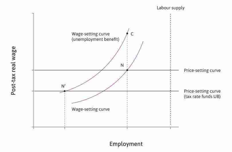
Short- and long-run effects of introducing an unemployment benefit.
Figure 8.34 Short- and long-run effects of introducing an unemployment benefit.
The unintended consequence
This raises the reservation option of employed workers, so that employers now have to pay more to induce workers to work hard and well. This is shown by point C.
Figure 8.34b This raises the reservation option of employed workers, so that employers now have to pay more to induce workers to work hard and well. This is shown by point C.
The result
The new Nash equilibrium is at N′, with higher unemployment.
Figure 8.34c The new Nash equilibrium is at N′, with higher unemployment.
We can summarize the impact of the policy:
- Short-run impact shifts the wage-setting curve upwards: The unemployed receive higher benefits and the employed receive higher wages (point C).
- Long-run impact is higher structural unemployment: There is a new Nash equilibrium in the long run. The economy is at point N′. As intended, the unemployed now receive higher income when out of work. But fewer workers are employed, which was not intended.
Unemployment benefits in the model and in the data
Surprisingly, when we look at the data, we find that countries with more generous unemployment benefits do not, on average, have higher unemployment rates. In Figure 8.35, for example, Sweden has quite generous unemployment benefits and a relatively low level of unemployment. This is even more the case for Norway, Denmark, and the Netherlands.
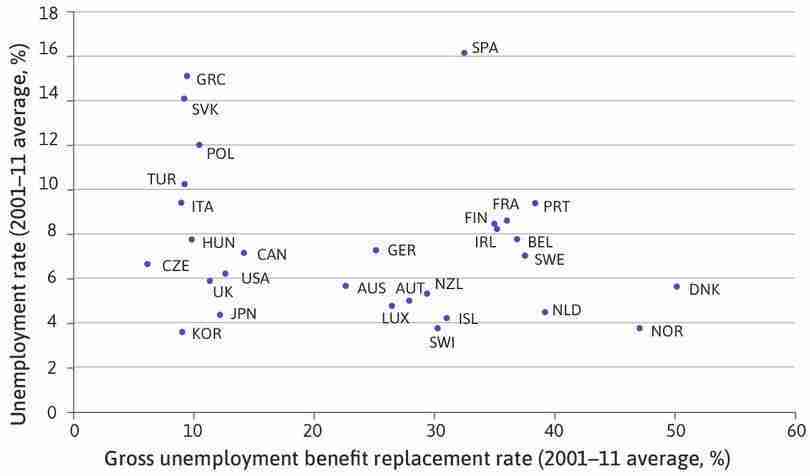
Unemployment benefit generosity and unemployment rates across the OECD (2001–2017).
Figure 8.35 Unemployment benefit generosity and unemployment rates across the OECD (2001–2017).
OECD (2019). OECD Statistics.
Unemployment benefits, unions, and wage-setting in Sweden
This suggests that these countries were able to achieve a Nash equilibrium outcome different from either N or N′. Figure 8.36 shows how this may have happened—there is a third Nash equilibrium at N″, where a new higher price-setting curve intersects the post reform wage-setting curve.
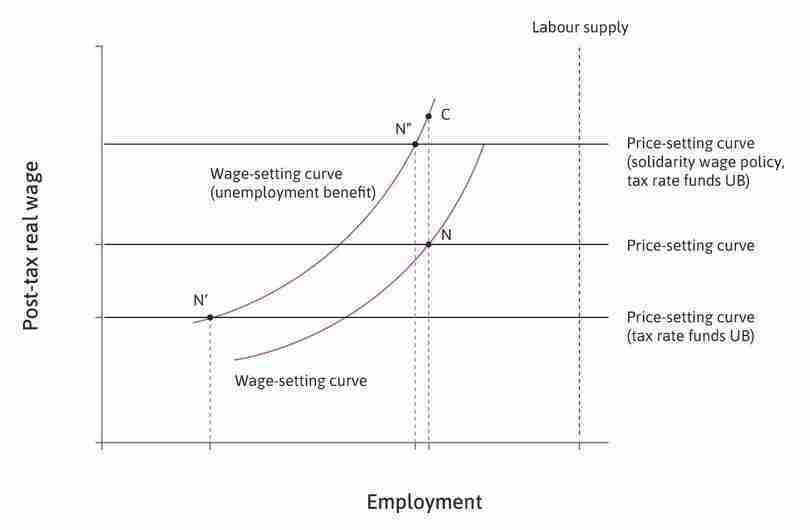
Combining the introduction of an unemployment benefit with a solidarity wage policy to raise productivity in the economy.
Figure 8.36 Combining the introduction of an unemployment benefit with a solidarity wage policy to raise productivity in the economy.
The Swedish approach had its origins in the ‘solidarity wage policy’, devised in 1951 by Gösta Rehn and Rudolph Meidner, two economists who worked at the research institute of the Trade Union Confederation in Sweden.
They reasoned that workers and employers have a common interest in rapid productivity growth, and that workers could enjoy higher wages without the profits of firms being reduced if more of the economy’s output was produced by high-productivity firms rather than by firms with low productivity.
In our ‘Economist in action’ video, John Van Reenen uses the game of cricket to explain how the economy’s average productivity is affected by the survival of low productivity firms.
The solidarity wage policy in Sweden was actually three linked policies:
- Equal wages for equal work: This means that the wage for each job was set at the national level by negotiations between the employers’ association and the union. This had the effect of reducing wage differences among workers doing similar jobs. The lowest-productivity firms had survived by paying lower wages than other firms paid to equivalent workers. Under the new policy, these firms could not pay the negotiated wage and still remain profitable, so they had to exit the industry. Higher-productivity firms survived and took over the market share of the failed firms.
- Unemployment benefits: These were generous but were only available for a relatively short time.
- Active labour market policy: Retraining and mobility allowances helped displaced workers find new jobs.
The solidarity wage policy forced low-productivity firms out of the market. The remaining firms had higher productivity and could, therefore, maintain their profit margins at lower prices, pushing the price-setting curve upwards. Retraining and mobility allowances ensured that these high-productivity firms had access to a well-trained workforce, allowing them to cut costs and prices even further.
Figure 8.36 shows how this combination of policies results in a new equilibrium with higher real wages at N″, and without the rise in unemployment at N′.
Question 8.11 Choose the correct answer(s)
Referring to Figure 8.36, which of the following statements are true?
- Real wages would remain at the level they were before the policy was introduced and employment would decrease.
- The price-setting curve is horizontal; therefore, unless the price-setting curve moves up or down, any equilibrium will have real wages at the same level.
- Imposing a standard wage for the job through national wage negotiations led to firms with productivity levels below the new negotiated wage exiting the industry.
- Unemployment benefits offer valuable insurance to workers who could lose their jobs. While workers are clearly made worse off by the decrease in employment, they may still benefit overall from the policy.
8.15 Looking backward: Baristas and bread markets
We have devoted much of this unit to the labour market for two reasons:
- It is important to society: If the labour market works well, the economy better serves our interests.
- It does not function like a price-taking market: It is essential to know the differences to understand how the economy as a whole works.
A good way to review these differences is to contrast the market for bread—used in the previous unit to illustrate the model of a competitive equilibrium of price-takers—with the market for, say, baristas (who, for readers unfamiliar with Italian-inspired coffee shops, are those who make espresso-based coffee drinks).
Taking a price, setting a price
Recall that, in the equilibrium of the bread market, neither bread consumers nor bakeries selling bread could benefit by offering to pay a different price or setting a different price from the one that prevailed in other transactions throughout the market. Buyers and sellers were price-takers in equilibrium:
- No (bread) buyer could benefit from offering to pay less than the prevailing price: No bakery would agree to the sale.
- No buyer could benefit by offering to pay more than the going price: This would just be throwing away money. Buyers in the bread market are price-takers because they wish to purchase bread at the lowest possible price.
- No seller (bakery) could benefit from setting a higher price: There would be no customers.
- No seller could benefit by offering a lower price: This would be throwing away money. Sellers can have as many customers as they like, at the existing price.
Now think about a buyer in the labour market. This is an employer who buys the employee’s time. The price is the wage. An employer who acts like a bread buyer would offer the employee the lowest wage that the individual would accept to take the job. This lowest possible wage is the reservation wage.
We know from Unit 6 that an employer who did this would be disappointed. The worker who is paid just a reservation wage does not worry about losing the job, and so would have little incentive to work hard. Instead, we saw that employers choose a wage to balance their wage costs against the positive effects of a higher wage on the employee’s motivation to work.
Complete and incomplete contracts
In the bread market, the sales contract between buyer and seller is for bread; if you buy bread you get what you want. It’s a complete contract (remember, a contract need not be in writing and it need not be signed to be enforceable—your receipt is enough to get a refund if the bag labelled ‘fresh bread’ turned out to contain a week-old loaf when you got home).
- incomplete contract
- A contract that does not specify, in an enforceable way, every aspect of the exchange that affects the interests of parties to the exchange (or of any others affected by the exchange).
In contrast, in the labour market, the employment contract is usually for the employee’s work time and not for the work itself. Because it is the employee’s work that produces the firm’s goods and is essential to the firm’s profits, this means the contract is an incomplete contract: something that matters to one of the parties to the exchange is not covered in the contract.
The implication is that, in contrast to the bread market, a buyer in the labour market is not throwing money away by paying more than is necessary to buy the employee’s time; it is the way that employers get what they want (work) and how they make profits. And because employers are deciding on the wage that they will offer the worker, they are wage-setters and not price-takers. This is why Unit 7’s model of the competitive equilibrium of price-takers does not work in the labour market.
Pareto efficiency and unexploited opportunities for mutual gains
- Pareto efficient
- An allocation with the property that there is no alternative technically feasible allocation in which at least one person would be better off, and nobody worse off.
- prisoners’ dilemma
- A game in which the payoffs in the dominant strategy equilibrium are lower for each player, and also lower in total, than if neither player played the dominant strategy.
- public goods game
- Similar to a prisoners’ dilemma game with more than two people; the dominant strategy is not to contribute to the public good.
In Unit 3, you encountered many situations in which the Nash equilibrium of some social interaction is not Pareto efficient. Examples include the prisoners’ dilemma and the public goods games.
- We use the Nash equilibrium: This concept helps us predict what outcomes we will observe when people interact.
- We use Pareto efficiency: This concept evaluates whether there is some other outcome in which all parties might have done better (or at least as well).
Recall from the model used to illustrate the bread market in Unit 7 that there were no unexploited opportunities for mutual gain at the competitive equilibrium (where the demand and supply curves intersect). In this situation, it is not possible to make one of the buyers or sellers better off without making at least one of them worse off. Therefore, the outcome was Pareto efficient.
This is not the case in the labour market. Competition among many buyers (firms hiring employees) and sellers (people seeking work) results in an equilibrium outcome—the wage w* and the level of employment N* —that is not Pareto efficient. What this means is that there is some other outcome—a different wage and level of employment that is feasible from the standpoint of the available resources and technology—that both employers and employees would prefer.
To see this, imagine that we are at the equilibrium of the labour market and product market (intersection of the wage-setting and price-setting curve at w* and N*), and one of the unemployed workers (identical to those employed) goes to an employer and says: ‘Give me a break. I’ll work as hard as the rest of your workforce, but you can pay me a little less.’
The employer thinks: ‘If I pay him a slightly lower wage, and if he works as hard as the rest, then my profits will go up.’
For the unemployed worker, getting a job makes a big difference. She now receives an employment rent, which measures how much better it is for her to have a job than not. The deal is a good one for her despite the fact that the employment rent she receives is slightly lower than that received by other workers (because her wage is slightly lower).
This example shows that there is some other technically feasible outcome—employ N* + 1 workers at the wage w* for N* of them and w* minus a little bit for the last worker hired—that would be an improvement for both the unemployed worker and the employer. Therefore, the outcome (N*, w*) is Pareto inefficient.
Why not hire a worker who is prepared to take a lower wage?
But if that is the case, why doesn’t the employer hire the unemployed person?
The answer is that the deal, while technically feasible, is not economically possible. This is because there is no way to enforce the unemployed person’s promise to work as hard as the rest in return for a slightly lower wage. Remember the w* on the wage-setting curve is the minimum the firm can pay to identical workers to ensure they work rather than shirk.
The problem, therefore, goes back to a fundamental fact about the relationship between the firm and its employees—the contract is incomplete in that it cannot ensure a given level of effort from the worker. The Nash equilibrium in the labour market is Pareto inefficient.
The politics and sociology of markets
Here is another difference between the bread market and the barista market. The baker probably does not know the name of the person buying the bread, or anything about the buyer other than that he is offering the right price for the loaf. The buyer most likely cares equally little about the baker, other than the taste of the bread.
Now think about the barista. What are the chances that he does not know the name of his immediate supervisor? And vice versa?
- employment relationship
- The interaction between an employee and an employer in which the employer sets the hours and other conditions of work and the wage, directs the employee’s activities and may terminate her employment, and the employee chooses how hard to work and whether to quit her job. The employee’s level of effort, or her decision to remain in the firm, are determined by the choices made by the two parties—and are affected by the exercise of power by the employer and the social norms of both parties.
Why the difference? The bread market tends to be a one-off interaction among virtual strangers, while the labour market is an ongoing interaction among people who not only know each other’s names, but also care about what the other person is like. We call it the employment relationship.
The barista’s supervisor cares about what the barista is like because his personality, loyalty to the brand, and his respect for social norms—such as honesty and hard work—influence the quality and quantity of effort that he puts into the job. The buyer of the bread does not care about these aspects of the baker because what matters is the quality of the loaf—which can be easily determined—and a new bakery readily found if the taste is not right.
Another major difference is that the supervisor directs what the barista does—to dress a certain way, to show up at work at a certain time, and to not waste time on the job—with the expectation that he will comply with her orders. Because the barista receives an employment rent that he would lose if the supervisor were to dismiss him, the supervisor can exercise power over him, getting him to do things that he might not do without the threat of dismissal.
This is not the case in the bread market. If the buyer complains about the baker’s attire, he would be invited to shop elsewhere. The difference is that neither the buyer nor the seller in the bread market is receiving a rent. For each of them, the transaction yields benefits virtually identical to the next best alternative. When both can walk away (selling to another customer; buying from another vendor) at virtually no cost, neither can exercise power over the other.
These are some of the differences—both economic and also political and sociological—between the bread market and the barista market. These are also the reasons why the model of the bread market with price-taking buyers and sellers and market clearing in equilibrium, does not work for the labour market. The table in Figure 8.37 summarizes the differences.
| Market | Bread: A market clearing equilibrium of price-takers | Baristas: Wage-setting by employers and equilibrium unemployment |
|---|---|---|
| Buyers | Individual consumers | Firms (employers) |
| Sellers | Firms (shops) | Individual workers |
| What is sold? | A loaf of bread | The worker’s time |
| What does the buyer want? | A loaf of bread | The employee’s effort on the job; not the worker’s time |
| Competition among sellers? | Yes: There are many bakeries competing to sell bread. | Yes: There are many actual or would-be baristas competing to sell their time. |
| Is the contract complete? | Yes: If the bag labelled bread did not contain bread, you get your money back. | No: The firm’s profits depend on the worker’s effort per hour/week/month worked, which is not in the contract. |
| Price-taking buyers? | Yes: Individual buyers cannot bargain for a lower price than others are willing to pay (and would not want to pay more). | No: The buyer (the firm) sets the wage to minimize the cost of getting the worker to work; it cannot benefit by offering the lowest wage at which the worker (the seller) would accept the job. |
| Is there excess supply or demand in equilibrium? | No: The market clears. Sales take place at the lowest price the seller would accept. | Yes: Firms offer a wage higher than the worker’s reservation wage (minimum price the seller would accept) to maximize their profits. |
Differences between the labour market and competitive (price-taking) product markets.
Figure 8.37 Differences between the labour market and competitive (price-taking) product markets.
Question 8.12 Choose the correct answer(s)
Which of the following statements are correct?
- In a competitive goods market, if what you buy is not what is advertised, then you can pursue the seller in court to ensure that the contract is fulfilled. In a labour market, the contract is for the employee’s work time, and not for the work (or the effort) itself, and therefore it is incomplete.
- In a competitive goods market, individual buyers cannot bargain for a lower price than others are willing to pay. Therefore, they are price-takers. In the labour market, the firms set the wage to minimize the cost of getting the worker to work; firms would not benefit by offering the lowest wage at which the worker (the seller) would accept the job. Hence, firms are price-setters.
- In a competitive goods market, the buyer’s next best alternative is to buy at another shop, while the seller’s next best alternative is to sell to another customer. Neither party is any worse off from leaving and, therefore, neither receives economic rents. In contrast, in the labour market the sellers (the employees) are worse off in their alternative of being unemployed. Hence, they receive employment rents.
- In goods markets, contracts are enforced, if necessary, by courts and not by norms. On the other hand, in labour markets the employees’ work ethic and/or feelings of reciprocity towards their employer affect their productivity on the job.
8.16 Structural and cyclical unemployment: The role of demand
Look back at Figure 8.17. There are large changes in the rate of unemployment relative to its long-term average (much more so in Spain than in Germany). It seems unlikely that the Nash equilibrium rate of unemployment in our model for Spain would drop precipitously from the late 1990s to the first five years of this century, and then jump back up five years later. It looks like more is going on in the unemployment data than is captured in our model.
Another case in point. At the beginning of this unit, you read about the father and son working in the Australian minerals sector (Doug and Rob Grey). The boom and bust in their lives reflected changes in economic conditions in the Australian economy as a whole. The minerals boom had produced the large-scale construction of mining facilities in Western Australia, Queensland, and the Northern Territory. As construction was coming to an end on existing projects, global iron ore prices collapsed, with the result that work was not started on new mines, ports, and processing facilities. In Figure 8.1, unemployment began to rise as the global price of iron ore plummeted.
Demand fluctuates and causes cyclical unemployment
Unemployment increased because the demand for labour in mining and in the related service activities shrank. Not only did the demand for minerals fall, but demand also declined for the goods and services that the Grey family and others like them would have purchased if they had kept their jobs. As a result, demand for goods and services fell across the economy, and with it the derived demand for labour. The term ‘derived demand for labour’ is used to highlight the fact that the firms’ demand for labour depends on the demand for their goods and services.
- cyclical unemployment
- The increase in unemployment above equilibrium unemployment caused by a fall in aggregate demand associated with the business cycle. Also known as: demand-deficient unemployment. See also: equilibrium unemployment.
Aggregate demand is the sum of the demand for all of the goods and services produced in the economy, whether from consumers, firms, the government, or buyers in other countries. The increase in unemployment caused by a fall in aggregate demand is called ‘demand-deficient’ unemployment—or, cyclical unemployment.
Observed unemployment is the sum of the cyclical unemployment and the level of unemployment at the Nash equilibrium of the labour market and product market, where the wage-setting and price-setting curves intersect (the structural unemployment):
Because the observed unemployment may fall below the equilibrium level—as it did during the mineral resources boom in Australia that underpinned the ‘good times’ for the Grey family—cyclical unemployment may be a negative number.
Cyclical and structural unemployment
How does this cyclical unemployment appear in our model of the economy, and how does it relate to structural unemployment?
Follow the analysis in Figure 8.38 to compare unemployment at the Nash equilibrium (at X) with the unemployment caused by a low level of aggregate demand (at B).
An unemployed person at X is involuntarily unemployed because that person would accept a job at the real wage shown by the intersection of the wage- and price-setting curves.
Notice that an unemployed person at point B is also involuntarily unemployed. In fact, such a person would accept a job with a wage below the wage shown at B, and would still be willing to work hard on the job.
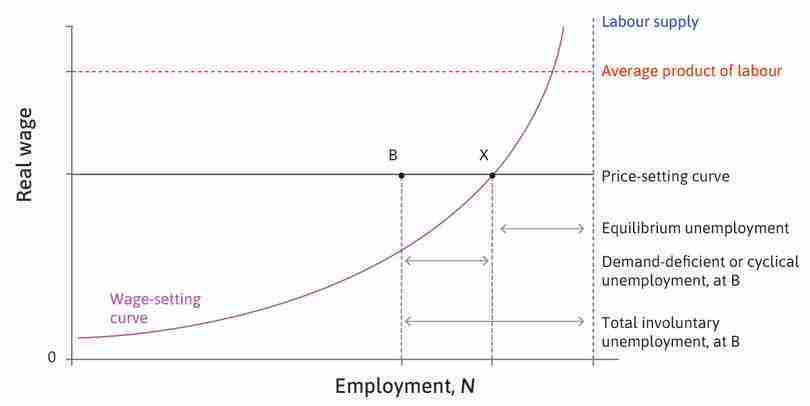
Equilibrium (structural) and demand-deficient (cyclical) unemployment.
Figure 8.38 Equilibrium (structural) and demand-deficient (cyclical) unemployment.
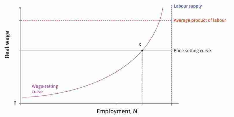
Point X
At X, unemployment is at its labour market equilibrium level. Someone losing a job at X is not indifferent between being employed and unemployed because that person experiences a cost of losing the job.
Figure 8.38a At X, unemployment is at its labour market equilibrium level. Someone losing a job at X is not indifferent between being employed and unemployed because that person experiences a cost of losing the job.
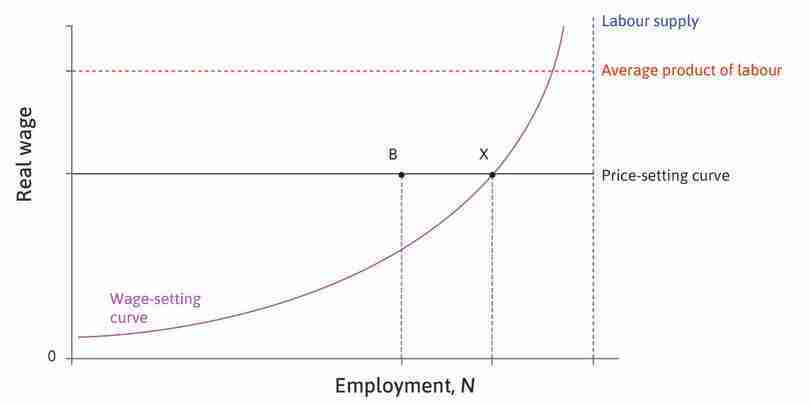
Point B
At B, there are additional people looking for work who are also involuntarily unemployed. The additional unemployment at B is due to low aggregate demand and is called demand-deficient, or cyclical, unemployment. They would be prepared to accept a lower wage, as long as it is not lower than the wage shown by the wage-setting curve. But without higher demand for their output, firms will not offer such jobs.
Figure 8.38b At B, there are additional people looking for work who are also involuntarily unemployed. The additional unemployment at B is due to low aggregate demand and is called demand-deficient, or cyclical, unemployment. They would be prepared to accept a lower wage, as long as it is not lower than the wage shown by the wage-setting curve. But without higher demand for their output, firms will not offer such jobs.
The Nash equilibrium
At point B, total involuntary unemployment is given by the sum of cyclical and structural unemployment.
Figure 8.38c At point B, total involuntary unemployment is given by the sum of cyclical and structural unemployment.
To find out more about using the WS/PS model to understand business cycles, inflation and unemployment, see Units 13-17 in the Core Economics website team’s The Economy, and Macroeconomics: Institutions, Instability and the Financial System by Wendy Carlin and David Soskice.
Question 8.13 Choose the correct answer(s)
Look again at Figure 8.38. Denote employment at point B as NB, employment at X as NX, and the total labour supply as NL. Which of the following statements about Figure 8.38 are correct?
- The demand-deficient unemployment is the increase in unemployment caused by the fall in aggregate demand, which is NX – NB.
- The firms’ demand for labour depends on the demand for their goods and services. These are NX at X and NB at B.
- At both B and X, all the unemployed workers are not out of work voluntarily.
- The equilibrium level of unemployment is NL – NX; any unemployment above this is demand-deficient (cyclical) unemployment.
8.17 Conclusion
The model of the aggregate economy presented here the (WS/PS model) brings together four decisions:
- workers deciding how hard to work
- owners of firms, through their HR department, deciding what wages to pay
- owners of firms, through their marketing department, deciding what prices to charge for their goods
- customers deciding how much to buy.
The relationships among the four actors and their four decisions are depicted in Figure 8.39.
Though the marketing and HR departments of the firm make decisions independently, they are unified under the direction of the firm’s owner who directs each to make decisions that will maximize his profits. Similarly, the customers and the employees may be the same people, or be members of the same family unified under their desire to have what they consider to be a good life.
The WS/PS model places all four decisions under a single lens and asks how the economy works as a result of their interactions. It identifies levels of real wages and structural unemployment that are consistent with the decisions taken independently by each of these decision-makers, that is the Nash equilibrium of the model.
The WS curve shifts downwards if:
- unemployment benefits decrease
- disutility of working decreases
- social stigma of unemployment increases
- technology lowers the cost of monitoring the worker’s effort.
The PS curve shifts downwards if:
- labour productivity decreases
- the markup increases as the result of markets being less competitive.
Trade unions can have different effects depending on size, bargaining power and behaviour:
- Bargained wage effect: How far the bargained WS curve lies above the employer-set curve depends on unions’ relative bargaining power, which is also influenced by laws and social norms.
- Union voice effect: The reciprocation of worker-friendly policies that reduce the disutility of effort shifts the best response curve as workers exert more effort.
- Labour productivity effect: By fostering a cooperative culture with management and encouraging productivity improvements unions can shift the PS curve.
The model of the aggregate economy allows us to chart the effect of changes in labour productivity, the extent of competition and the institutions governing the relationship between employers and employees not only on wages and employment but also on the degree of inequality in the economy as a whole using the Lorenz curve and Gini coefficient.
8.18 Doing Economics: Measuring the non-monetary cost of unemployment
In Section 8.7, we explained why there will always be involuntary unemployment in labour market equilibrium, in order to create an employment rent that motivates employed workers. The employment rent takes into account both monetary and non-monetary costs and benefits, such as social status from being employed. On the other hand, being unemployed may be psychologically as well as financially detrimental because of the stress of looking for a new job, as well as social norms and expectations regarding work.
In Doing Economics Empirical Project 8, we will use self-reported wellbeing to measure the disutility from unemployment, and see whether social norms can explain any differences in wellbeing between the employed and unemployed in European countries.
Go to Doing Economics Empirical Project 8 to work on this project.
Learning objectives
In this project you will:
- practise working with fairly large datasets
- detect and correct entries in a dataset
- re-code variables to make them easier to analyse
- calculate percentiles for subsets of the data
- calculate confidence intervals for the difference in means between groups.
8.19 References
- Carlin, Wendy, and David Soskice. 2015. Macroeconomics: Institutions, Instability, and the Financial System. New York, NY: Oxford University Press.
- Freeman, Sunny. 2015. ‘What Canada can learn from Sweden’s unionized retail workers’. Huffington Post Canada Business. Updated 19 March 2015.
- Hirsch, Barry T. 2008. ‘Sluggish institutions in a dynamic world: Can unions and industrial competition coexist?’ Journal of Economic Perspectives 22 (1) (February): pp. 153–76.
- The Core Economics website team. The Economy. New York, NY: Oxford University Press.
-
Sunny Freeman. 2015. ‘What Canada can learn from Sweden’s unionized retail workers’. Huffington Post Canada Business. Updated 19 March 2015. ↩
-
Barry T. Hirsch. 2008. ‘Sluggish institutions in a dynamic world: Can unions and industrial competition coexist?’ Journal of Economic Perspectives 22 (1) (February): pp. 153–76. ↩
