5 Institutions, power, and inequality
5.1 Introduction
- Institutions influence the balance of power among conflicting people or groups and affect the resulting level of inequality and other outcomes.
- Technology, biology, and people’s preferences are also important determinants of economic outcomes.
- Power is the ability to do and get the things one wants in opposition to the intentions of others.
- Interactions between economic actors can result in mutual gains, but also in conflicts over how the gains are distributed, which affect inequality.
- Institutions influence the power and other bargaining advantages of actors.
- The degree of inequality can be measured and compared, both across societies and historical periods, and before and after the implementation of public policies.
Perhaps one of your distant ancestors considered that the best way to get money was by going to sea with a pirate like Blackbeard or Captain Kidd. If he had settled on Captain Bartholomew Roberts’ pirate ship the Royal Rover, he and the other members of the crew would have been required to consent to the ship’s written constitution. Figure 5.1 shows what the ship’s constitution (called The Royal Rover’s Articles) guaranteed.
The example of the Royal Rover is taken from a fascinating article on the economic consequences of being a pirate. Peter T. Leeson. 2007. ‘An-arrgh-chy: The Law and Economics of Pirate Organizations’. Journal of Political Economy 115 (6): pp. 1049–94.
Peter T. Leeson. 2007. ‘An-arrgh-chy: The Law and Economics of Pirate Organizations’. Journal of Political Economy 115 (6): pp. 1049–94.
The Royal Rover and its Articles were not unusual. During the heyday of European piracy in the late seventeenth and early eighteenth centuries, most pirate ships had written constitutions that guaranteed even more powers to the crew members. Their captains were democratically elected (‘the Rank of Captain being obtained by the Suffrage of the Majority’). Many captains were also voted out, at least one for cowardice in battle. Crews also elected one of their number as the quartermaster who, when the ship was not in a battle, could countermand the captain’s orders.
If your ancestor had served as a lookout and had been the first to spot a ship that was later taken as a prize, he would have received as a reward ‘the best Pair of Pistols on board, over and above his Dividend’. Were he to have been seriously wounded in battle, the articles guaranteed him compensation for the injury (more for the loss of a right arm or leg than for the left). He would have worked as part of a multiracial, multi-ethnic crew, of which probably about a quarter were of African origin, and the rest primarily of European descent, including Americans.
The result was that a pirate crew was often a close-knit group. A contemporary observer lamented that the pirates were ‘wickedly united, and articled together’. Sailors of captured merchant ships often happily joined the ‘roguish Commonwealth’ of their pirate captors.
Another unhappy commentator remarked: ‘These Men whom we term … the Scandal of human Nature, who were abandoned to all Vice … were strictly just among themselves.’ If they were Responders in the ultimatum game that we explained in Unit 3, Section 3.3, by this description they would have rejected any offer less than half of the pie!
5.2 Institutions: The rules of the game
In the late seventeenth and early eighteenth centuries, there was no country in the world that ordinary workers had the right to vote, to receive compensation for occupational injuries, or to be protected from arbitrary authority. These rights were taken for granted on the Royal Rover.
The Royal Rover’s Articles laid down the understandings among the pirates about their working conditions. They determined who did what aboard the ship, and what each person would get. For example, the size of the helmsman’s dividend compared to that of the gunner. There were also unwritten informal rules of appropriate behaviour that the pirates followed by custom, or to avoid condemnation by their crewmates, or punishment by the captain or quartermaster.
- institution
- The laws and social customs governing the way people interact in society.
How the pirates interacted with one another was governed by their institutions.
Recall that institutions are the written and unwritten rules that regulate how people interact: this includes who meets whom, who does what tasks, with what rewards or penalties. On the Royal Rover, one rule was that the best pair of pistols would be given to the lookout who spotted a ship that was later taken. Another was that the captain and quartermaster would receive two shares, and ordinary crew one share, of the booty.
Private property is an economic institution that (as you learned in Unit 1), gives the owner of some object (a home, for example) the right to exclude others from its use, and to sell it to someone else.
Political institutions determine how a person may come to be a head of state (for example, a royal position inherited from a parent, or by election), and the kinds of things that government officials are permitted or prohibited from doing (for example, entering a private home without invitation or permission from the court system). Democracy (as you know from Unit 1) is an institution.
Marital institutions regulate who may marry whom (and who may not) as well as practices concerning the raising of children and the inheritance of property across generations. Monogamy—one spouse per person—is an institution. Primogeniture, under which inheritance passes to the eldest offspring—usually throughout history the eldest son—is another.
Two things to keep in mind about how we use the term ‘institution’:
- Organizations are not institutions: In common parlance, large organizations such as the University of Oxford and the Hyundai Motor Company are sometimes referred to as institutions. We will call an entity with a proper name an ‘organization’, and reserve the word ‘institution’ for a set of rules of the game, not for any particular example of those rules at work.
- Institutions include social norms as well as laws: Institutions can be formal (written and enforced) or informal. An example of a formal institution is the rule in football (soccer) that only goalkeepers may touch the ball with their hands while the ball is in play. An informal institution is the convention or social norm that if Team A kicks the ball off the pitch because there is an injury to a player on Team B, Team B always returns the ball to Team A from the restart. This is not written in any rule book and yet it is widely accepted, although less so in recent years. It is a social norm.
Institutions in models
Because we use games to represent how people interact, we naturally use the term ‘rules of the game’ to mean the same thing as ‘institutions’.
Institutions directly affect inequality—the extent to which some people have more and others have less—as you can see by re-reading the Royal Rover’s constitution.
- bargaining power
- The extent of a person’s advantage in securing a larger share of the economic rents made possible by an interaction.
The rules of the ultimatum game that you studied in Unit 3 determine the ability of the players to obtain a high payoff (the extent of their advantage when dividing the pie), which is called bargaining power. A Proposer’s right to make a take-it-or-leave-it offer gives her more bargaining power than the Responder, and usually results in the Proposer getting more than half of the pie.
Still, the Proposer’s bargaining power is limited because the Responder has the power to refuse. Suppose we allow a Proposer simply to divide up a pie in any way, without any role for the Responder other than to take whatever he gets (if anything). Under these rules, the Proposer has all the bargaining power and the Responder none. There is an experimental game like this, called (you guessed it) the dictator game. ‘Dictators’ in this game typically make a lot more money than Proposers in the ultimatum game.
In experiments, the assignment of the role Proposer or Responder, and hence the assignment of bargaining power, is usually done by chance. In real economies, the assignment of power is definitely not random.
Institutions and power
In the labour market, the power to set the terms of the exchange typically lies with those who own the business—they are the ones proposing the wage and other terms of employment. Those seeking employment are like Responders, and since usually more than one person is applying for the same job, their bargaining power may be low. Also, because the place of employment is the employer’s private property, the employer may be able to exclude the worker by firing her if her work is not up to the employer’s specifications.
There are many past and present examples of economic institutions that are like the dictator game, in which there is no option to say no. Examples include today’s remaining political dictatorships, such as The Democratic People’s Republic of Korea (North Korea), and slavery, as it existed in the US prior to the end of the American Civil War in 1865.
Criminal organizations involved in drugs and human trafficking are another modern example, in which power takes the form of physical coercion or threats of violence. The term ‘modern slavery’ refers to relationships that migrants and sex workers are sometimes subject to, in which the worker is bound to the employer by physical threats, the employer seizing the worker’s passport, and by other coercive means.
In a democratic society, however, institutions exist to protect people against violence and coercion, and to ensure that most economic interactions are conducted voluntarily.
As we saw in Unit 1, India became a democracy in 1948. To provide a concrete case of institutions and how they change, we now look at how legislation in 1978 changed the institutions governing how a crop would be divided between the farmer who cultivated the land and the owner of the land.
How Operation Barga changed the rules of the game
In the Indian state of West Bengal, home to more people than Germany, many farmers work as sharecroppers (‘bargadars’ in the Bengali language), renting land from landowners in exchange for a share (that is, a percentage) of the crop.
The traditional contractual arrangements throughout this vast state varied little from village to village, with virtually all bargadars giving half their crop to the landowner at harvest time. This had been the social norm for at least five centuries.
But in the second half of the twentieth century many thought this was unfair, because of the extreme levels of deprivation among the bargadars. In 1973, 73% of the rural population lived in poverty, one of the highest poverty rates in India. The state and national government had generally supported the landlords. But in 1978, a democratic state election altered the balance of political power. The newly elected Left Front government of West Bengal adopted new laws, called Operation Barga.
The new laws benefited bargadars:
- They could keep three-quarters of their crop: The landlords’ share was cut from one-half to one-quarter.
- They were protected from eviction by landowners: They were protected as long as they paid the newly legislated rent (one-quarter of the crop).
Both provisions of Operation Barga were advocated as a way of increasing output. There are certainly reasons to predict that the size of the pie would increase, as well as the incomes of the farmers:
- They had a greater incentive to work hard and well: Keeping a larger share meant that there was a greater reward if they grew more crops.
- They had an incentive to invest in improving the land: They were confident that they would farm the same plot of land in the future, so would be rewarded for their investment.
Did this dramatic change in institutions work?
Because the new law was implemented over many years, one village at a time (there are more than 20,000 villages in the state), economists have been able to isolate the effect of Operation Barga from other changes that were occurring at the same time (the weather, for example). By comparing the output of farms before and after the implementation of Operation Barga, researchers concluded that it improved work motivation, and increased investment.
One study estimated that Operation Barga was responsible for about 28% of the subsequent growth in output per farmer in the region. The empowerment of the bargadars also had positive spill-over effects as local governments became more responsive to the needs of poor farmers.1
The result was that West Bengal experienced a dramatic increase in farm output per unit of land, as well as rising farming incomes.
Efficiency and fairness
Operation Barga was later cited by the World Bank as an example of good policy for economic development.2
The evidence from Operation Barga indicates that, in this case, the pie got larger, and the poorest people got a larger slice.
- Pareto criterion
- According to the Pareto criterion, a desirable attribute of an allocation is that it be Pareto efficient. See also: Pareto dominant.
In principle, the increase in the size of the pie means there could be mutual gains from the reforms, with both farmers and landowners being better off. In other words, there could be an improved allocation, according to the Pareto criterion as discussed in Section 3.3.
The actual change in the allocation was not a Pareto improvement, however—landlords had strenuously opposed the legislation, but the bargadars and their allies far outnumbered them, so the Left Front’s political power was secure in India’s democratic political system. The incomes of some landowners fell following the legislated reduction in their share of the crop. Nevertheless, in increasing the income of the poorest people in West Bengal, many would judge that Operation Barga implemented an improvement in the allocation from the standpoint of fairness. We can assume that many people in West Bengal thought so, because they continued to vote for the Left Front alliance. It stayed in power from 1977 until 2011.
Operation Barga illustrates an important fact—institutions affect who has power, and this matters for who gets more and who gets less from the economy. To understand how institutions (the rules of the game) and the exercise of power affect the degree of inequality and other economic outcomes, we now present a model of that process.
Question 5.1 Choose the correct answer(s)
Which of the following statements about institutions are correct?
- In economic terms, institutions do not refer to organizations or the buildings they occupy, but rather refers to the rules of the game that specify who can do what, when they can do it, and how each player’s actions determine their payoff.
- Institutions can be written (for example, constitutions) or unwritten (for example, social norms that determine what behaviour is considered appropriate).
- Institutions determine who can do what, and how payoffs are distributed.
- In economics, institutions are defined as the rules of the game that specify who can do what, when they can do it, and how each player’s actions determine their payoff.
Question 5.2 Choose the correct answer(s)
Which of the following statements regarding bargaining power are correct?
- In an ultimatum game, the Responder has the power to refuse the Proposer’s offer (resulting in a zero payoff for the Proposer). This gives the Responder some bargaining power.
- Increasing the number of Responders reduces their power to refuse (as the other Responder(s) may accept). This increases the Proposer’s bargaining power.
- In a dictator game, the Responder has no role other than to take whatever is offered, if anything. Therefore, the Responder has no bargaining power and the Proposer has all the bargaining power.
- In a dictator game, the Proposer has all the bargaining power irrespective of the number of Responders, who have no role other than to take whatever is offered, if anything.
5.3 Production and distribution: Using a model
Recall the model in Unit 4 of the farmer, Angela, who produces a crop. We will extend that model by introducing a sequence of scenarios involving two characters, Angela and Bruno. We introduce them as people and we personify what they do and are trying to accomplish, even reporting on their conversations. We use two characters and the institutions governing how they interact to illustrate general facts about an entire society composed of many Angelas and Brunos. This story is an economic model simplifying reality to convey something important about how the much more complex world works.
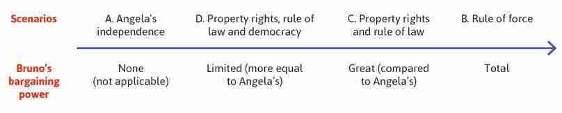
Their story unfolds over a period of time in which they live under differing sets of institutions—different scenarios—as shown in the table (Figure 5.2). As you can see in the first scenario, Bruno is not in the picture and Angela gets everything she produces. In deciding how hard to work, she is facing a problem identical to the one we presented in Unit 4. Next, we consider three scenarios involving Bruno, the owner of the land on which Angela works. In scenarios B, C, and D, what will happen—how many hours she will work and how much of what she produces she will get—depends on the ways in which the institutions characterizing these three scenarios give more or less bargaining power to Angela and Bruno.
| Scenario | In the model of Angela and Bruno | In the real world |
|---|---|---|
| A | Independence: Angela works the land on her own, and everything she produces is hers. | Independent farmers with access to land (either free, or because they own it) have been common in history ever since farming began. |
| B | Rule of force: Slavery. There is a second person, who does not farm, but is able to take some of the harvest. He is called Bruno. Bruno is heavily armed, and Angela is, effectively, his slave. | Also common throughout history: slavery and other forms of coerced labour in mines and plantations was the basis of much of the economy of North and South America after the arrival of Europeans. It persists today—among domestic workers and sex workers—though in most countries illegally. In the UK for example, the Modern Slavery Act was passed in 2015. |
| C | Property rights and the rule of law: Laws protect Angela from coercion but give Bruno ownership of the land. If she wants to farm his land, she must agree, for example, to pay him some part of the harvest. But she has the right to say no. He has to make her an offer that she will accept. | In manufacturing, farming, and other kinds of work, owners of land and other capital goods employ workers, or make their land available to the landless for rent, a common arrangement today and for thousands of years. The sharecropping in Bengal in India is an example. |
| D | Property rights, the rule of law, and the right to vote: the rules of the game are a bit more in Angela’s favour. She and her fellow farmers achieve the right to vote and legislation is passed that increases Angela’s claim on the harvest. | Capitalism and democracy in the twentieth century and today. Operation Barga in Bengal changed the rules and was the result of political pressure in a democracy. |
Institutional arrangements in a model and in the world.
Figure 5.2 Institutional arrangements in a model and in the world.
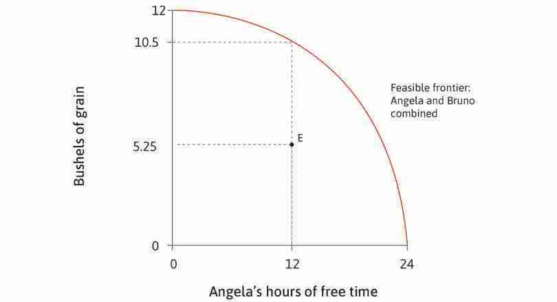
In Figure 5.3, we depict how much bargaining power Bruno has over Angela.
Bruno’s bargaining power over Angela depends on the institutions in force in the four scenarios.
Figure 5.3 Bruno’s bargaining power over Angela depends on the institutions in force in the four scenarios.
For each of these scenarios, we will analyse the changes in terms of both Pareto efficiency and the distribution of income between Angela and Bruno. Remember that:
- Pareto efficient
- An allocation with the property that there is no alternative technically feasible allocation in which at least one person would be better off, and nobody worse off.
- indifference curve
- A curve of the points which indicate the combinations of goods that provide a given level of utility to the individual.
- marginal rate of substitution (MRS)
- The trade-off that a person is willing to make between two goods. At any point, this is the slope of the indifference curve. See also: marginal rate of transformation.
- If we have enough facts, we can probably agree on whether an outcome is Pareto efficient or not.
- Whether or not the outcome is fair depends on your own assessment of the problem, using the concepts of substantive and procedural fairness introduced in Unit 3.
Angela values both grain and free time. Again, we represent her preferences as indifference curves, showing the combinations of grain and free time that she values equally. Remember that the slope of the indifference curve is called the marginal rate of substitution (MRS) between grain and free time.
An independent producer: Angela farms the land on her own
Figure 5.4 shows Angela’s indifference curves and her feasible frontier. Remember: the indifference curves are about what Angela values. The feasible frontier is about what she can get. The steeper the indifference curve, the more Angela values free time relative to grain. You can see that the more free time she has (moving to the right), the flatter the curves—she values free time less.
In this unit, we make a particular technical assumption about Angela’s preferences that you can see in the shape of her indifference curves. If she gets more grain, but her hours of free time do not change, then her MRS does not change either. For example, as you move up the vertical line at 16 hours of free time, the slope of each indifference curve crossing the line is the same. More grain does not change her valuation of free time relative to grain.
To simplify the graphical exposition of the model, we assume that preferences are quasi-linear. To explore this further using calculus, see Leibniz 5.4.1 from The Economy.
Why might this be? Perhaps she does not eat it all, but sells some and uses the proceeds to buy other things she needs. This is just a simplification that makes our model easier to understand. When drawing indifference curves for the model in this unit, remember to simply shift them up and down, keeping the MRS constant at a given amount of free time.
Angela is free to choose her typical hours of work to achieve her preferred combination of free time and grain. Go through the analysis of Figure 5.4 to determine the allocation.
- marginal rate of transformation (MRT)
- A measure of the trade-offs a person faces in what is feasible. Given the constraints (feasible frontier) a person faces, the MRT is the quantity of some good that must be sacrificed to acquire one additional unit of another good. At any point, it is the slope of the feasible frontier. See also: feasible frontier, marginal rate of substitution.
Figure 5.4 shows that the best Angela can do, given the limits set by the feasible frontier, is to work for 8 hours. She has 16 hours of free time and produces and consumes 9 bushels of grain. This is the number of hours of work where the marginal rate of substitution is equal to the marginal rate of transformation. She cannot do better than this! (If you’re not sure why, go back to Unit 4 and check.)
Question 5.3 Choose the correct answer(s)
Based on Figure 5.4, which of the following statements are correct?
- The MRS is the trade-off between grain and free time that Angela is willing to make.
- To the left of Angela’s optimal choice, the slope of her indifference curve (MRS) is steeper than the slope of the feasible frontier (MRT). Therefore, the MRS is greater than the MRT.
- To the right of Angela’s optimal choice, the slope of her indifference curve is less steep than at C, so she is less willing to trade grain for free time.
- Even though MRS = MRT at those points inside the frontier, the only optimal choice is on the feasible frontier, since Angela is on her highest indifference curve, given her constraint, so she is doing the best that she can.
5.4 The rule of force: Bruno appears and has unlimited power over Angela
Angela now has company. The other person is called Bruno. He is not a farmer but is heavily armed and can claim some—even all—of Angela’s harvest. We will study different rules of the game that explain how much is produced by Angela, and how it is divided between her and Bruno. For example, in one scenario, Bruno is the landowner and Angela pays some grain to him as rent for the use of the land. But we start with the rule of force.
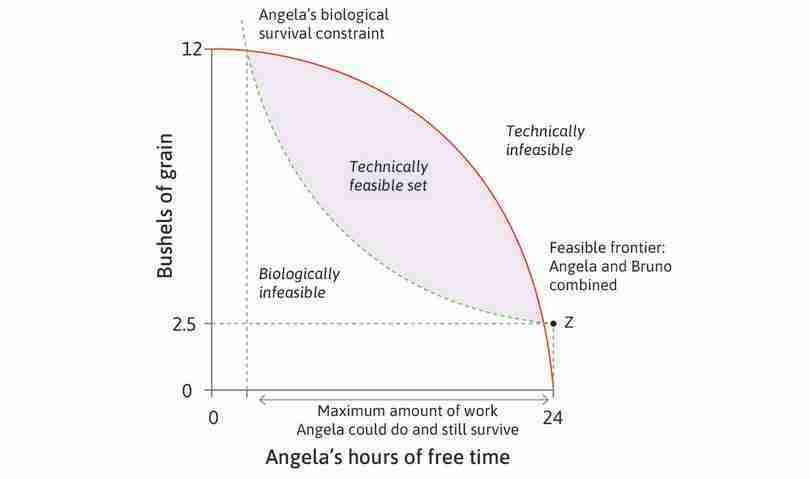
Figure 5.5 shows Angela and Bruno’s combined feasible frontier. The frontier indicates how many bushels of grain Angela can produce given how much free time she takes. For example, if she takes 12 hours of free time and works for 12 hours, then she produces 10.5 bushels of grain. One possible outcome of the interaction between Angela and Bruno is that 5.25 bushels go to Bruno, and Angela retains the other 5.25 bushels for her own consumption.
Work through the analysis of Figure 5.5 to find out how each possible allocation is represented in the diagram, showing how much work Angela does and how much grain she and Bruno each get.
Feasible outcomes of the interaction between Angela and Bruno.
Figure 5.5 Feasible outcomes of the interaction between Angela and Bruno.
The combined feasible frontier
The feasible frontier shows the maximum amount of grain available to Angela and Bruno together, given Angela’s amount of free time. If Angela takes 12 hours of free time and works for 12 hours, then she produces 10.5 bushels of grain.
Figure 5.5a The feasible frontier shows the maximum amount of grain available to Angela and Bruno together, given Angela’s amount of free time. If Angela takes 12 hours of free time and works for 12 hours, then she produces 10.5 bushels of grain.
A feasible allocation
Point E is a possible outcome of the interaction between Angela and Bruno.
Figure 5.5b Point E is a possible outcome of the interaction between Angela and Bruno.
The distribution at point E
At point E, Angela works for 12 hours and produces 10.5 bushels of grain. The distribution of grain is such that 5.25 bushels go to Bruno and Angela retains the other 5.25 bushels for her own consumption.
Figure 5.5c At point E, Angela works for 12 hours and produces 10.5 bushels of grain. The distribution of grain is such that 5.25 bushels go to Bruno and Angela retains the other 5.25 bushels for her own consumption.
Other feasible allocations
Point F shows an allocation in which Angela works more than at point E and gets less grain. Point G shows the case in which she works more and gets more grain.
Figure 5.5d Point F shows an allocation in which Angela works more than at point E and gets less grain. Point G shows the case in which she works more and gets more grain.
An impossible allocation
An outcome at H—in which Angela works for 12 hours a day, Bruno consumes the entire amount produced and Angela consumes nothing—which would not be possible; she would starve.
Figure 5.5e An outcome at H—in which Angela works for 12 hours a day, Bruno consumes the entire amount produced and Angela consumes nothing—which would not be possible; she would starve.
Which allocations are likely to occur? Not all of them are even possible. For example, at point H Angela works for 12 hours a day and receives nothing (Bruno takes the entire harvest), so Angela would not survive. Of the allocations that are at least possible, the one that will occur depends on the rules of the game.
Question 5.4 Choose the correct answer(s)
Based on Figure 5.5, which of the following statements are correct?
- Angela’s indifference curves are downward-sloping. If the indifference curve through G was sufficiently flat, the other three points would all lie below it.
- Whatever the slope of her indifference curves, Angela would prefer E to F, as it gives her more grain and more free time.
- Bruno gets an amount of grain equal to the vertical distance from the allocation to the feasible frontier. Therefore, G is the worst of the four allocations for him.
- Angela could be indifferent between G and E—one of her indifference curves could pass through both points.
Exercise 5.1 An allocation you have known
Think of a job that you or someone you know has done (for example, a barista or an office worker).
- Who are the parties involved in this economic interaction?
- Describe the allocation—who does what, and who gets what?
- Do you think the allocation is fair? Explain your answer.
How much can Bruno get?
As an independent farmer, Angela could consume (or sell) everything she produced. Now Bruno has arrived. He has the power to implement any allocation that he chooses. He is even more powerful than the dictator in the dictator game (in which a Proposer dictates how a pie is to be divided). Why? Bruno can determine the size of the pie, as well as how it is shared.
Unlike the experimental subjects in Unit 3, in this model Bruno and Angela are entirely self-interested. Bruno wants only to maximize the amount of grain he can get. Angela cares only about her own free time and grain (as described by her indifference curves), just as she did in Unit 4.
- reservation option
- A person’s next best alternative among all options in a particular transaction. Also known as: fallback option. See also: reservation price.
We now make another important assumption. If Angela does not work the land, Bruno gets nothing (there are no other prospective farmers that he can exploit). What this means is that Bruno’s reservation option (what he gets if Angela does not work for him) is zero. As a result, Bruno thinks about the future—he will not take so much grain that Angela will starve. The allocation must keep her alive and physically able to work.
- biologically feasible
- An allocation that is capable of sustaining the survival of those involved is biologically feasible.
Angela’s biological survival constraint in Figure 5.6 shows the minimum amount of grain that she needs for each amount of work that she does; points below this line would leave her so undernourished or overworked that she would not survive. This constraint shows what is biologically feasible. Notice that, if she expends more energy working, she needs more food; that’s why the curve rises from right to left from point Z as her hours of work increase. The slope of the biological survival constraint is the marginal rate of substitution between free time and grain in securing Angela’s survival.
The fact that Angela’s survival might be in jeopardy is not a hypothetical example. During the Industrial Revolution, life expectancy at birth in Liverpool, UK, fell to 25 years—slightly more than half of what it is today in the poorest countries in the world. In many parts of the world today, farmers’ and workers’ capacity to do their jobs is limited by their intake of calories.
The biological survival constraint tells us the least amount that Angela can get under Bruno’s rule of force while continuing to exist. But this constraint need not literally be biological. If Angela is receiving too little, she might choose to try to escape to a place where she could farm her own land and keep the entire crop. Or she might prefer the risk of trying to get his gun. In either case her relationship to him as a forced worker would change, just as if she had starved.
This extension of our model in which Angela takes action rather than submitting to the rule of force is not hypothetical. Rebellions of slaves and slaves driven to attempt escape because of their conditions are common in the history of that institution. They are probably more common than stories of starvation: slave owners had an interest in keeping a slave strong enough to work hard.
So, you can think of what we term the biological constraint as a sustainability constraint where what is being sustained is the relationship of forced labour between the two.
- technically feasible
- An allocation within the limits set by technology and biology.
Next, we will work out the set of technically feasible combinations of Angela’s hours of work and the amount of grain she receives—that is, all the combinations that are possible within the limitations of the technology (the production function) and biology (Angela must have enough nutrition to do the work and survive).
Figure 5.6 shows how to find the technically feasible set. We already know that the production function determines the feasible frontier. This is the technological limit on the total amount consumed by Bruno and Angela, which in turn depends on the hours that Angela works.
Technically feasible allocations.
Figure 5.6 Technically feasible allocations.
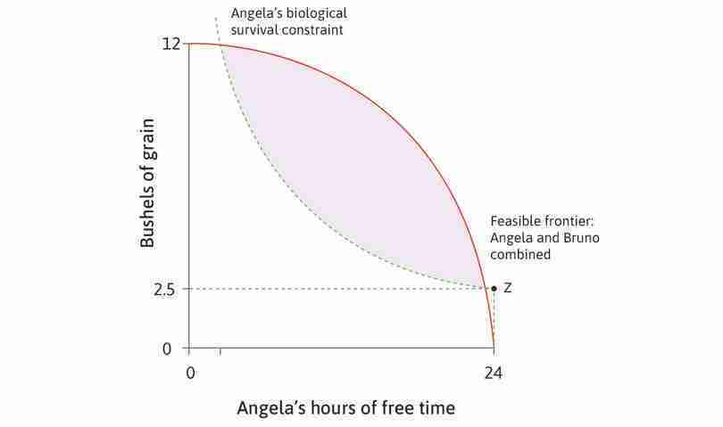
The biological survival constraint
If Angela does not work at all, she needs 2.5 bushels to survive (point Z). If she gives up some free time and expends energy working, she needs more food, so the curve is higher when she has less free time. This is the biological survival constraint.
Figure 5.6a If Angela does not work at all, she needs 2.5 bushels to survive (point Z). If she gives up some free time and expends energy working, she needs more food, so the curve is higher when she has less free time. This is the biological survival constraint.
Biologically infeasible and technically infeasible points
Points below the biological survival constraint are biologically infeasible, while points above the feasible frontier are technically infeasible.
Figure 5.6b Points below the biological survival constraint are biologically infeasible, while points above the feasible frontier are technically infeasible.
Angela’s maximum working day
Given the feasible frontier, there is a maximum amount of work above which Angela could not survive, even if she could consume everything she produced.
Figure 5.6c Given the feasible frontier, there is a maximum amount of work above which Angela could not survive, even if she could consume everything she produced.
The technically feasible set
The technically feasible allocations are the points in the lens-shaped area bounded by the feasible frontier and the biological survival constraint (including points on the frontier).
Figure 5.6d The technically feasible allocations are the points in the lens-shaped area bounded by the feasible frontier and the biological survival constraint (including points on the frontier).
If Angela could consume everything she produced (the height of the feasible frontier) and choose her hours of work, her survival would not be in jeopardy, since the biological survival constraint is below the feasible frontier for a wide range of working hours. The question of biological feasibility arises because of Bruno’s claims on her output.
In Figure 5.6, the boundaries of the feasible solutions to the allocation problem are formed by the feasible frontier and the biological survival constraint. This lens-shaped area gives the technically possible outcomes. We can now ask what will actually happen—which allocation will occur, and how does this depend on the institutions governing Bruno’s and Angela’s interaction?
Question 5.5 Choose the correct answer(s)
Based on Figure 5.6, which of the following statements are correct?
- At 24 hours of work (or 0 hours of free time), Angela’s biological survival constraint is above the feasible frontier. This means that, at this point, she cannot produce enough grain to survive.
- Angela would not produce any grain if she did not work. This is not technically feasible because she needs 2 bushels of grain to survive.
- Technology that boosted grain production would increase the amount of grain that could be produced for any given number of working hours, shifting the feasible frontier up and thus expanding the technically feasible set.
- If Angela did not need as much grain to survive, the biological survival constraint would be lower, making the technically feasible set bigger.
Given his power, Bruno makes his choice
With the help of his gun, Bruno can choose any point in the lens-shaped technically feasible set of allocations. But which will he choose?
He reasons like this:
- Bruno
- For any number of hours that I order Angela to work, she will produce the amount of grain shown by the feasible frontier. But I’ll have to give her at least the amount shown by the biological survival constraint for that much work, so that I can continue to exploit her. I get to keep the difference between what she produces and what I give her. Therefore, I should find Angela’s working hours for which the vertical distance between the feasible frontier and the biological survival constraint (Figure 5.6) is the greatest.
Bruno first considers letting Angela continue to work for 8 hours a day, producing 9 bushels, as she did when she had free access to the land. For 8 hours of work, she needs 3.5 bushels of grain to survive. Therefore, Bruno could take 5.5 bushels without jeopardizing his future opportunities to benefit from Angela’s labour.
Bruno is studying Figure 5.6 and asks for your help. You have noticed that at 8 hours of work the MRS on the survival constraint is less than the MRT.
- You
- Bruno, your plan cannot be right. If you forced her to work a little more, she’d only need a little more grain to have the energy to work longer, because the biological survival constraint is relatively flat at 8 hours of work. But the feasible frontier is steep, so she would produce a lot more if you imposed longer hours.
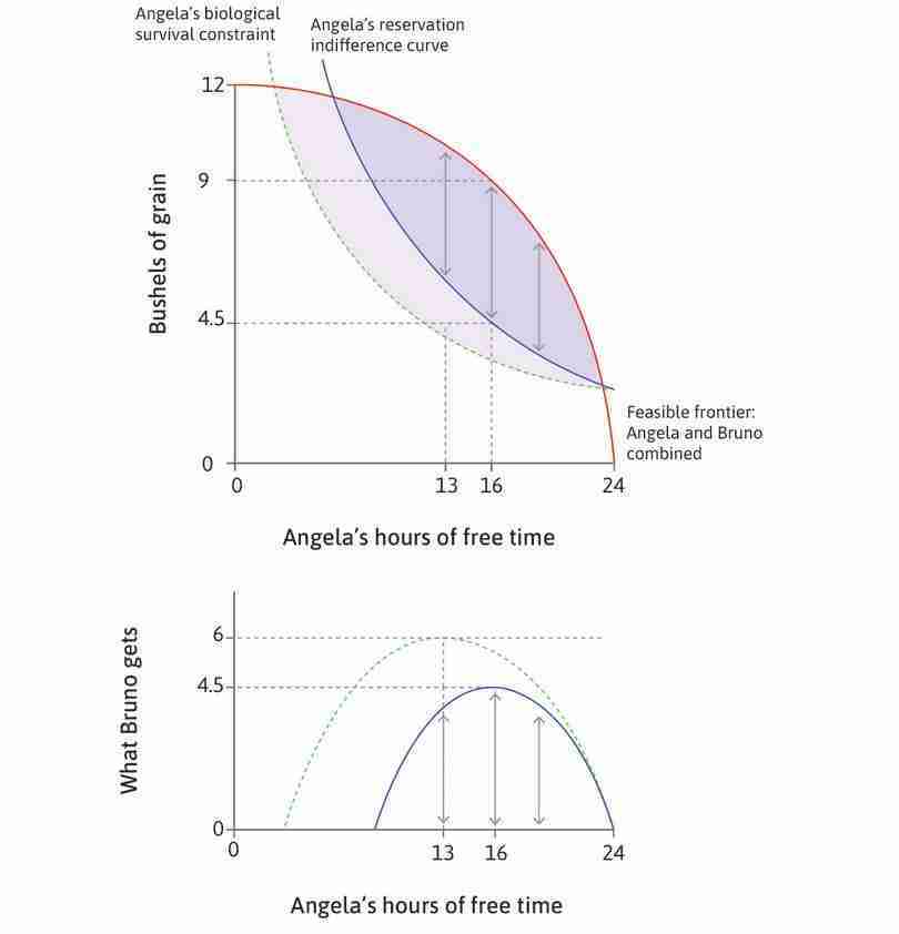
You demonstrate the argument to him using the analysis in Figure 5.7, which indicates that the vertical distance between the feasible frontier and the biological survival constraint is the greatest when Angela works for 11 hours (13 hours of free time). If Bruno commands Angela to work for 11 hours, then she will produce 10 bushels and Bruno will get to keep 6 bushels for himself. We can use Figure 5.7 to find out how many bushels of grain Bruno will get for any technically feasible allocation.
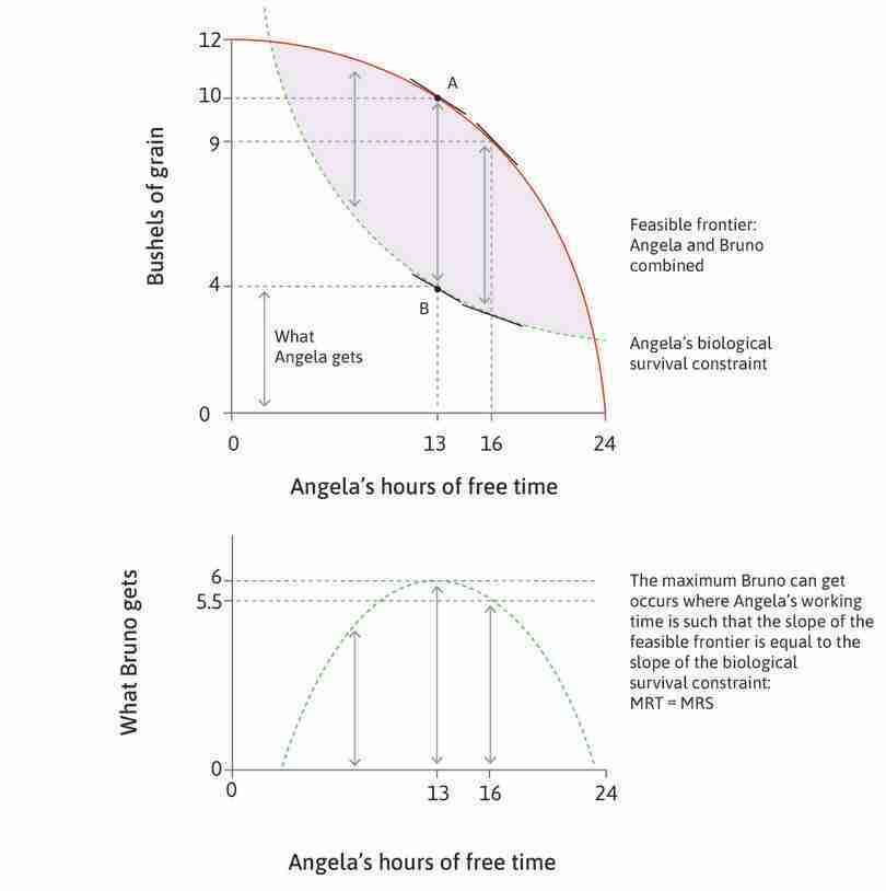
Scenario B: Coercion. The maximum technically feasible transfer from Angela to Bruno.
Figure 5.7 Scenario B: Coercion. The maximum technically feasible transfer from Angela to Bruno.
Bruno can command Angela to work
Bruno can choose any allocation in the technically feasible set. He considers letting Angela continue working for 8 hours a day, producing 9 bushels.
Figure 5.7a Bruno can choose any allocation in the technically feasible set. He considers letting Angela continue working for 8 hours a day, producing 9 bushels.
When Angela works for 8 hours
Bruno could take 5.5 bushels without jeopardizing his future benefit from Angela’s labour. This is shown by the vertical distance between the feasible frontier and the survival constraint.
Figure 5.7b Bruno could take 5.5 bushels without jeopardizing his future benefit from Angela’s labour. This is shown by the vertical distance between the feasible frontier and the survival constraint.
The maximum distance between frontiers
The vertical distance between the feasible frontier and the biological survival constraint is greatest when Angela works for 11 hours (13 hours of free time).
Figure 5.7c The vertical distance between the feasible frontier and the biological survival constraint is greatest when Angela works for 11 hours (13 hours of free time).
Allocation and distribution at the maximum distance
If Bruno commands Angela to work for 11 hours, she will produce 10 bushels, and needs 4 to survive. Bruno will get to keep 6 bushels for himself (the distance AB).
Figure 5.7d If Bruno commands Angela to work for 11 hours, she will produce 10 bushels, and needs 4 to survive. Bruno will get to keep 6 bushels for himself (the distance AB).
The best Bruno can do for himself
Bruno gets the maximum amount of grain by choosing allocation B, where Angela’s working time is such that the slope of the feasible frontier is equal to the slope of the biological survival constraint: MRT = MRS.
Figure 5.7g Bruno gets the maximum amount of grain by choosing allocation B, where Angela’s working time is such that the slope of the feasible frontier is equal to the slope of the biological survival constraint: MRT = MRS.
The lower panel in the last step in Figure 5.7 shows how the amount Bruno can take varies with Angela’s free time. The graph is hump-shaped, and peaks at 13 hours of free time and 11 hours of work. Bruno maximizes his amount of grain at allocation B, commanding Angela to work for 11 hours.
- economic rent
- A payment or other benefit received above and beyond what the individual would have received in his or her next best alternative (or reservation option). See also: reservation option.
Notice how the slopes of the feasible frontier and the survival constraint (the MRT and MRS) help us to find the number of hours where Bruno can take the maximum amount of grain. To the right of 13 hours of free time (that is, if Angela works for less than 11 hours), the biological survival constraint is flatter than the feasible frontier (MRS < MRT). This means that working more hours (moving to the left) would produce more grain than Angela needs for the extra work. To the left of 13 hours of free time (Angela working more), the reverse is true—MRS > MRT. Bruno’s economic rent is greatest at the hours of work where the slopes of the two frontiers are equal.
That is:
Question 5.6 Choose the correct answer(s)
Based on Figure 5.7, if Bruno can impose the allocation:
- At the technically feasible point where Angela produces the most grain, she needs all the grain to survive, so there would be none for Bruno.
- The distance between the feasible frontier and Angela’s survival constraint, and thus Bruno’s share, is maximized where MRS = MRT.
- At 8 hours of work (16 hours of free time) the feasible frontier is steeper than the biological survival constraint. Thus MRT > MRS.
- Bruno would indeed choose 13 hours of free time for Angela, but the maximum he can claim without making Angela unable to work is 6 bushels of grain—the vertical distance between the feasible frontier and the survival constraint.
5.5 Property rights and the rule of law
- private property
- The right and expectation that one can enjoy one’s possessions in ways of one’s own choosing, exclude others from their use, and dispose of them by gift or sale to others who then become their owners.
- power
- The ability to do (and get) the things one wants in opposition to the intentions of others, ordinarily by imposing or threatening sanctions.
In the previous section, Bruno had the power to enslave Angela. If we move from a scenario of coercion to one in which there is a legal system that prohibits slavery and protects private property and the rights of landowners and workers, we can expect the outcome of the interaction to change.
In the example above, Angela was forced to participate, and Bruno chose her working hours to maximize his own economic rent. Next, we look at the situation where she can simply say no. Angela is no longer a slave, but Bruno still has the power to make a take-it-or-leave-it offer, just like the Proposer in the ultimatum game.
In Unit 1, we defined private property as the right to use and exclude others from the use of something, and the right to sell it (or to transfer these rights to others). From now on, we will suppose that Bruno owns the land and can exclude Angela if he chooses. How much grain he will get as a result of his private ownership of the land will depend on the extent of his power over Angela in the new situation.
The rule of law arrives and Angela can say no
We check back on Angela and Bruno, and immediately notice that Bruno is now wearing a suit and is no longer armed, at least not openly. He explains that his weapon is no longer needed because there is a government with laws administered by courts, and professional enforcers, called the police. Bruno now owns the land, and Angela must have permission to use his property. He can offer a contract allowing her to farm the land, and she can give him part of the harvest in return. But the law requires that exchange is voluntary—Angela can refuse the offer.
- Bruno
- It used to be a matter of power, but now both Angela and I have property rights—I own the land, and she owns her own labour. The new rules of the game mean that I can no longer force Angela to work. She has to agree to the allocation that I propose.
- You
- And if she doesn’t?
- Bruno
- Then there is no deal. She doesn’t work on my land, I get nothing, and she gets barely enough to survive from the government.
- You
- So you and Angela have the same amount of power?
- Bruno
- Certainly not! I am the one who gets to make a take-it-or-leave-it offer. I am like the Proposer in the ultimatum game, except that this is no game. If she refuses, she goes hungry.
- You
- But if she refuses, you get zero?
- Bruno
- That will never happen.
Why does he know this? Bruno knows that Angela, unlike the real subjects in the ultimatum game experiments, is entirely self-interested (she does not punish an unfair offer). If he makes an offer that is just a tiny bit better for Angela than not working at all and getting subsistence rations, she will accept it.
Now he asks you a question similar to the one he asked earlier.
- Bruno
- In this case, what should my take-it-or-leave-it offer be?
You answered before by showing him the biological survival constraint. Now the limitation is not Angela’s survival, but rather her agreement. You know that she values her free time, so the more hours he offers her to work, the more he is going to have to pay.
- You
- Why don’t you just look at Angela’s indifference curve that passes through the point where she does not work at all and barely survives? That will tell you how much is the least you can pay her for each of the hours of free time she would give up in order to work for you.
- reservation indifference curve
- A curve that indicates allocations (combinations) that are as highly valued as one’s reservation option. See also: reservation option.
Point Z in Figure 5.8 is the allocation in which Angela does no work and gets only survival rations (from the government, or perhaps her family). This is her reservation option—if she refuses Bruno’s offer, she has this option as a backup. Follow the analysis of Figure 5.8 to see Angela’s reservation indifference curve—all the allocations that have the same value for her as the reservation option. Below or to the left of the curve, she is worse off than in her reservation option. Above and to the right, she is better off.
Angela’s reservation indifference curve is above her biological survival constraint (except at point Z) because, at all points on the biological constraint, she might be close to starvation. The points differ in how many hours of free time she has. Being about to starve and not having to work is preferable to Angela than being about to starve and working 18-hour days. The points on her reservation indifference curve are combinations of free time and grain that are equally valued to Angela as doing no work and receiving 2.5 bushels of grain.
The set of points bounded by the reservation indifference curve and the feasible frontier, is the set of all economically feasible allocations now that Angela has to agree to Bruno’s proposal. Bruno thanks you for this handy new tool for figuring out the most he can get from Angela.
The biological survival constraint and the reservation indifference curve have a common point (Z)—at that point, Angela does no work and gets subsistence rations from the government. Other than that, the two curves differ. The reservation indifference curve is uniformly above the biological survival constraint. The reason, you explain to Bruno, is that, however hard she works along the survival constraint, she barely survives; and the more she works the less free time she has, so the unhappier she is. Along the reservation indifference curve, by contrast, she is just as well off as at her reservation option, meaning that being able to keep more of the grain that she produces compensates exactly for her lost free time.
We can see that both Angela and Bruno may benefit if a deal can be made. Their exchange—allowing her to use his land (that is, not using his property right to exclude her) in return for her sharing some of what she produces—makes it possible for both to be better off than if no deal had been struck:
- Bruno is better off than if there is no deal: This is true as long as Bruno gets some of the crop.
- Angela can also benefit: This is true as long as Angela’s share makes her better off than she would have been if she took her reservation option, taking account of her work hours.
This potential for mutual gain is why their exchange need not take place at the point of a gun but can be motivated by the desire of both to be better off.
At this point, you decide, it would make it a lot easier to explain the situation to Bruno, if he were familiar with some basic terms from economics.
Exercise 5.2 Biological and economic feasibility
Using Figure 5.8:
- Explain why a point on the biological survival constraint is higher (more grain is required) when Angela has fewer hours of free time. Why does the curve also get steeper when she works more?
- Explain why the biologically feasible set is not equal to the economically feasible set.
Explain (by shifting the curves) how you would represent the effects of the following:
- an improvement in growing conditions, such as more adequate rainfall
- Angela having access to half the land that she had previously
- Angela having a better-designed hoe, making it physically easier to do the work of farming.
An economics lesson for Bruno
- economic rent
- A payment or other benefit received above and beyond what the individual would have received in his or her next best alternative (or reservation option). See also: reservation option.
- gains from exchange
- The benefits that each party gains from a transaction compared to how they would have fared without the exchange. Also known as: gains from trade. See also: economic rent.
When people participate voluntarily in an interaction, they do so because they expect the outcome to be better than their reservation option—the next best alternative. The difference between the value of participating and the value of the next best alternative is called an economic rent. For example, if a deal with Angela results in Bruno getting 3 bushels of grain, he receives an economic rent of 3 bushels (since, if he does not interact with Angela, he gets nothing). Economic rents are also sometimes called gains from exchange, because they are how much a person gains by engaging in the exchange compared to not engaging.
- joint surplus
- The sum of the economic rents of all involved in an interaction. Also known as: gains from exchange.
The sum of the economic rents of the participants is termed the surplus (or sometimes the joint surplus, to emphasize that it includes all the rents). How much rent they will each get—how they will share the surplus—depends on their bargaining power. And that, as we know, depends on the institutions governing the interaction.
- Pareto improvement
- A change that benefits at least one person without making anyone else worse off. See also: Pareto dominant.
All the allocations that represent mutual gains are shown in the economically feasible set in Figure 5.8. Each of these allocations Pareto-dominates the allocation that would occur without a deal. In other words, Bruno and Angela could achieve a Pareto improvement.
This does not mean that both parties will benefit equally. If the institutions in effect give Bruno the power to make a take-it-or-leave-it offer subject only to Angela’s agreement, he can capture the entire surplus (minus the tiny bit necessary to get Angela to agree). Bruno knows this already.
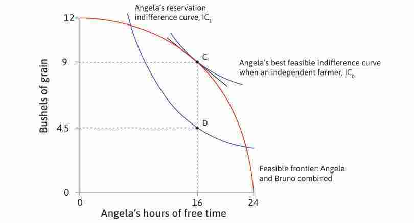
Once you have explained the reservation indifference curve to him, Bruno knows which allocation he wants. He maximizes the amount of grain he can get at the maximum height of the lens-shaped region between Angela’s reservation indifference curve and the feasible frontier. This is where the MRT on the feasible frontier is equal to the MRS on the indifference curve. Figure 5.9a shows that this allocation requires Angela to work for fewer hours than she did under coercion.
Scenario C: Bruno’s take-it-or-leave-it proposal when Angela can refuse.
Figure 5.9a Scenario C: Bruno’s take-it-or-leave-it proposal when Angela can refuse.
Bruno’s best outcome using coercion
Using coercion, Bruno chose allocation B. He forced Angela to work for 11 hours and received grain equal to AB. The MRT at A is equal to the MRS at B on Angela’s biological survival constraint.
Figure 5.9a-a Using coercion, Bruno chose allocation B. He forced Angela to work for 11 hours and received grain equal to AB. The MRT at A is equal to the MRS at B on Angela’s biological survival constraint.
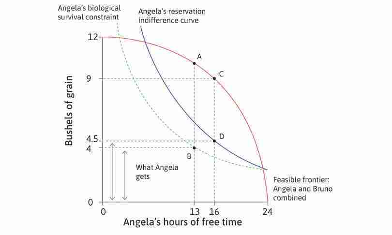
When Angela can say no
With voluntary exchange, allocation B is not available. The best that Bruno can do is allocation D, where Angela works for 8 hours, giving him grain equal to CD.
Figure 5.9a-b With voluntary exchange, allocation B is not available. The best that Bruno can do is allocation D, where Angela works for 8 hours, giving him grain equal to CD.
Bruno would like Angela to work for 8 hours and give him 4.5 bushels of grain (allocation D). How can he implement this allocation? All he has to do is to make a take-it-or-leave-it offer of a contract, allowing Angela to work the land in return for giving him a share of the crop equal to 4.5 bushels per day. (This is a sharecropping contract, like the bargadars’ contracts in West Bengal.) We could say that she rents the land from Bruno, but we will call the payment a crop share to avoid confusion between land rent and economic rent.
If Angela has to pay 4.5 bushels (CD in Figure 5.9a) then she will choose to produce at point C, where she works for 8 hours. You can see this in the figure; if she produced at any other point on the feasible frontier and then gave Bruno 4.5 bushels, she would have lower utility—she would be below her reservation indifference curve. But she can achieve her reservation utility by working for 8 hours, so she will accept the contract.
Exercise 5.3 Why Angela works for 8 hours
Angela’s income is the amount she produces minus the crop share she pays to Bruno.
- Using Figure 5.9a, suppose Angela works for 11 hours. Would her income (after paying Bruno) be greater or less than when she works for 8 hours? Suppose instead, she works for 6 hours, how would her income compare with when she works for 8 hours?
- Explain in your own words why she will choose to work for 8 hours.
Since Angela is on her reservation indifference curve, only Bruno benefits from this exchange. All the joint surplus goes to Bruno. His economic rent is the whole surplus.
Remember that, when Angela could work the land on her own, she chose allocation C. Notice now that she chooses the same hours of work when she has to pay Bruno. Why does this happen? Whatever the crop share Angela has to pay, she will choose her hours of work to maximize her utility, so she will produce at a point on the feasible frontier where the MRT is equal to her MRS. And we know that her preferences are such that her MRS doesn’t change with the amount of grain she consumes, so it will not be affected by the crop share. This means that, if she can choose her hours, she will work for 8 hours, irrespective of the crop share (as long as this gives her at least her reservation utility).
Figure 5.9b shows how the surplus (which Bruno gets) varies with Angela’s hours. You will see that the surplus falls as Angela works for more or less than 8 hours. It is hump-shaped, like Bruno’s rent in the case of coercion. But the peak is lower when Bruno needs Angela to agree to the proposal.
Scenario C: Bruno’s take-it-or-leave-it proposal when Angela can refuse.
Figure 5.9b Scenario C: Bruno’s take-it-or-leave-it proposal when Angela can refuse.
Angela’s working hours when she was coerced
Using coercion, Angela was forced to work for 11 hours. The MRT was equal to the MRS on Angela’s biological survival constraint.
Figure 5.9b-a Using coercion, Angela was forced to work for 11 hours. The MRT was equal to the MRS on Angela’s biological survival constraint.
Bruno’s best take-it-or-leave-it offer
When Bruno cannot force Angela to work, he should offer a contract in which Angela pays him 4.5 bushels to rent the land. She works for 8 hours, where the MRT is equal to the MRS on her reservation indifference curve.
Figure 5.9b-b When Bruno cannot force Angela to work, he should offer a contract in which Angela pays him 4.5 bushels to rent the land. She works for 8 hours, where the MRT is equal to the MRS on her reservation indifference curve.
Bruno’s grain
Although Bruno cannot coerce Angela, he can get the whole surplus.
Figure 5.9b-d Although Bruno cannot coerce Angela, he can get the whole surplus.
Technically and economically feasible peaks compared
The peak of the hump is lower when Angela can refuse, compared to when Bruno could order her to work.
Figure 5.9b-e The peak of the hump is lower when Angela can refuse, compared to when Bruno could order her to work.
Exercise 5.4 Take it or leave it?
- Why is it Bruno, and not Angela, who has the power to make a take-it-or-leave-it offer?
- Describe a situation in which the farmer, not the landowner, might have this power.
Question 5.7 Choose the correct answer(s)
Bruno is a landowner and Angela is a farmer who pays a share of her grain output to Bruno for the use of the land. Suppose that Angela works for 8 hours a day and produces 10 bushels of grain. Angela’s subsistence level of consumption is 4 bushels of grain. Based on this information, which of the following statements is correct?
- The surplus is the total rent, which in this case is 10 bushels. The relative bargaining power only determines how this surplus is shared between the two.
- The gains from exchange are the rents Bruno and Angela receive above their next-best alternative, which in this case is no production. If Angela had all the bargaining power, then her rent would be 10 bushels.
- The surplus is the total rent gained above the next-best alternative, which in this case is no production. Therefore, the surplus is 10 bushels.
- If Bruno claimed all 10 bushels, then Angela will be left with no grain. Since she needs at least 4 bushels of grain to survive, this allocation is not biologically feasible.
Question 5.8 Choose the correct answer(s)
Figure 5.9a shows Angela and Bruno’s feasible frontier, Angela’s biological survival constraint, and her reservation indifference curve. B is the outcome under coercion, while D is the outcome under voluntary exchange when Bruno makes a take-it-or-leave-it offer.
From this figure, we can conclude that:
- Bruno’s reservation option is to receive nothing. Under voluntary exchange, Bruno receives the whole of the surplus—the amount in excess of what Angela needs to either survive or be willing to work. This is his economic rent.
- Bruno’s amount of grain is the distance AB under coercion, and CD under voluntary exchange. Therefore, he is better off under coercion.
- Bruno offers an allocation Angela is only just willing to accept. She is indifferent between D and her reservation option, so her rent is zero.
- Angela will have more hours of free time under voluntary exchange than under coercion.
5.6 Efficiency and conflicts over the distribution of the surplus
Given that she had the right to say no, Angela chose to work for 8 hours, producing 9 bushels of grain, both when she had to pay a share of the crop to Bruno and also when she did not. In both cases, there is a surplus of 4.5 bushels—the difference between the amount of grain produced, and the amount that would give Angela her reservation utility.
The two cases differ in who gets the surplus. When Angela had to pay a crop share, Bruno took the whole surplus, but when she could work the land for herself, she obtained all the surplus. Both allocations have two important properties:
- All the grain produced is shared.
- MRS = MRT again: The MRT on the feasible frontier is equal to the MRS on Angela’s indifference curve.
- Pareto efficient
- An allocation with the property that there is no alternative technically feasible allocation in which at least one person would be better off, and nobody worse off.
This means that the allocations are Pareto efficient.
To see why, remember that Pareto efficiency means that it is impossible to change the allocation to make one party better off without making the other worse off; in other words, no Pareto improvement is possible.
The first property is straightforward—it means that no Pareto improvement can be achieved simply by changing the amounts of grain they each consume. If one consumed more, the other would receive less. On the other hand, if some of the grain produced was not being consumed, then consuming it would make one or both of them better off.
Pareto efficiency and the Pareto efficiency curve
- A Pareto-efficient allocation has the property that there is no alternative, technically feasible allocation in which at least one person would be better off, and nobody worse off.
- The set of all such allocations is the Pareto efficiency curve. It is also referred to as the contract curve.
The second property, MRS = MRT, means that no Pareto improvement can be achieved by changing Angela’s hours of work and hence the amount of grain produced.
If the MRS and MRT were not equal, it would be possible to make both better off. For example, if MRT > MRS, Angela could transform an hour of her time into more grain than she would need to get the same utility as before, so the extra grain could make both of them better off. But if MRT = MRS, then any change in the amount of grain produced would only be exactly what is needed to keep Angela’s utility the same as before, given the change in her hours.
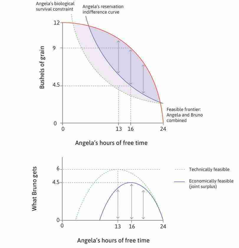
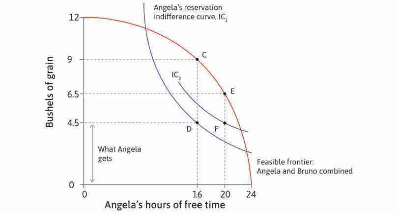
Figure 5.10 shows that there are many other Pareto-efficient allocations in addition to these two. Point C is the outcome when Angela is an independent farmer. Compare the analysis in Figure 5.10 with Bruno’s take-it-or-leave-it offer to see the other Pareto-efficient allocations.
Pareto-efficient allocations and the distribution of the surplus.
Figure 5.10 Pareto-efficient allocations and the distribution of the surplus.
The allocation at C
As an independent farmer, Angela chose point C, where MRT = MRS. She consumed 9 bushels of grain—4.5 bushels would have been enough to put her on her reservation indifference curve at D. But she obtained the whole surplus CD—an additional 4.5 bushels.
Figure 5.10a As an independent farmer, Angela chose point C, where MRT = MRS. She consumed 9 bushels of grain—4.5 bushels would have been enough to put her on her reservation indifference curve at D. But she obtained the whole surplus CD—an additional 4.5 bushels.
The allocation at D
When Bruno owned the land and made a take-it-or-leave-it offer, he chose a contract in which the crop share was CD (4.5 bushels). Angela accepted and worked for 8 hours. The allocation was at D, and once again, MRT = MRS. The surplus was still CD, but Bruno got it all.
Figure 5.10b When Bruno owned the land and made a take-it-or-leave-it offer, he chose a contract in which the crop share was CD (4.5 bushels). Angela accepted and worked for 8 hours. The allocation was at D, and once again, MRT = MRS. The surplus was still CD, but Bruno got it all.
Angela’s preferences
Remember that Angela’s MRS doesn’t change as she consumes more grain. At any point along the line CD, such as G, there is an indifference curve with the same slope. Therefore, MRS = MRT at all these points.
Figure 5.10c Remember that Angela’s MRS doesn’t change as she consumes more grain. At any point along the line CD, such as G, there is an indifference curve with the same slope. Therefore, MRS = MRT at all these points.
A hypothetical allocation
Point G is a hypothetical allocation, at which MRS = MRT. Angela works for 8 hours, and 9 bushels of grain are produced. Bruno gets grain CG, and Angela gets all the rest. Allocation G is Pareto efficient.
Figure 5.10d Point G is a hypothetical allocation, at which MRS = MRT. Angela works for 8 hours, and 9 bushels of grain are produced. Bruno gets grain CG, and Angela gets all the rest. Allocation G is Pareto efficient.
The Pareto efficiency curve
All the points making up the line between C and D are Pareto-efficient allocations, at which MRS = MRT. The surplus of 4.5 bushels (CD) is shared between Angela and Bruno.
Figure 5.10e All the points making up the line between C and D are Pareto-efficient allocations, at which MRS = MRT. The surplus of 4.5 bushels (CD) is shared between Angela and Bruno.
- Pareto efficiency curve
- The set of all allocations that are Pareto efficient. Often referred to as the contract curve, even in social interactions in which there is no contract, which is why we avoid the term. See also: Pareto efficient.
Figure 5.10 shows that, in addition to the two Pareto-efficient allocations we have observed (C and D), every point between C and D represents a Pareto-efficient allocation. CD is called the Pareto efficiency curve—it joins together all the points in the feasible set for which MRS = MRT. (You will also hear it called the contract curve, even in situations where there is no contract, which is why we prefer the more descriptive term Pareto efficiency curve.)
At each allocation on the Pareto efficiency curve, Angela works for 8 hours and there is a surplus of 4.5 bushels, but the distribution of the surplus is different—ranging from point D where Angela gets none of it, to point C where she gets it all. At the hypothetical allocation G, both receive an economic rent—Angela’s rent is GD, Bruno’s is GC, and the sum of their rents is equal to the surplus.
Question 5.9 Choose the correct answer(s)
Based on Figure 5.10, which of the following statements is correct?
- All points on CD are Pareto efficient, so none of them is Pareto-dominated. (Comparing C and D, we see that Bruno prefers D and Angela prefers C.)
- The Pareto efficiency curve, by definition, joins all the economically feasible points where MRS = MRT.
- All the points on CD are Pareto efficient. It does not make any sense to say that one point on CD is more efficient than another.
- All the points on CD are Pareto efficient, but Bruno and Angela are not indifferent. Some points (like C) are better for Angela, while others (like D) are better for Bruno.
5.7 Property rights, the rule of law, and the right to vote
Bruno thinks that the new rules, under which he makes an offer that Angela will not refuse, are not so bad after all. Angela is also better off than she had been when she had barely enough to survive. But she would like a share in the surplus.
Fairness: Changing the law by democratic means
Angela and her fellow farm workers lobby for a new law that limits working time to 4 hours a day, while requiring that total pay is at least 4.5 bushels. They threaten to not work at all unless the law is passed.
- Bruno
- Angela, you and your colleagues are bluffing.
- Angela
- No, we are not. We would be no worse off at our reservation option than under your contract, working the hours and receiving the small fraction of the harvest that you impose!
Angela and her fellow workers win, and the new law limits the working day to 4 hours.
How did things work out?
Before the short-hours law, Angela worked for 8 hours and received 4.5 bushels of grain. This is point D in Figure 5.11. The new law implements the allocation in which Angela and her friends work for 4 hours, getting 20 hours of free time and the same number of bushels. Since they have the same amount of grain and more free time, they are better off. Figure 5.11 shows they are now on a higher indifference curve.
Scenario D: The effect of an increase in Angela’s bargaining power through legislation.
Figure 5.11 Scenario D: The effect of an increase in Angela’s bargaining power through legislation.
Before the short-hours law
Bruno makes a take-it-or-leave-it offer, gets grain equal to CD, and Angela works for 8 hours. Angela is on her reservation indifference curve at D and MRS = MRT.
Figure 5.11a Bruno makes a take-it-or-leave-it offer, gets grain equal to CD, and Angela works for 8 hours. Angela is on her reservation indifference curve at D and MRS = MRT.
The effect of legislation
With legislation that reduces work to 4 hours a day and keeps Angela’s amount of grain unchanged, she is on a higher indifference curve at F. Bruno’s grain is reduced from CD to EF (2 bushels).
Figure 5.11c With legislation that reduces work to 4 hours a day and keeps Angela’s amount of grain unchanged, she is on a higher indifference curve at F. Bruno’s grain is reduced from CD to EF (2 bushels).
MRT > MRS
When Angela works for 4 hours, the MRT is larger than the MRS on the new indifference curve.
Figure 5.11d When Angela works for 4 hours, the MRT is larger than the MRS on the new indifference curve.
Angela’s economic rent
Angela’s economic rent can be measured, in bushels of grain, as the vertical distance between point J on her reservation indifference curve (IC1 in Figure 5.11) and point F on the indifference curve she is able to achieve under the new legislation (IC2).
Figure 5.11e Angela’s economic rent can be measured, in bushels of grain, as the vertical distance between point J on her reservation indifference curve (IC1 in Figure 5.11) and point F on the indifference curve she is able to achieve under the new legislation (IC2).
Angela and Bruno’s rents
To sum up, the introduction of the new law has increased Angela’s bargaining power and Bruno is worse off than before. You can see that she is better off at F than at D. Because she is better off than she would be with her reservation option, she is now receiving an economic rent.
Remember the term ‘economic rent’ does not mean what you pay to your landlord, it means what you are getting above what you would get in your reservation position. Bruno’s reservation position (if Angela runs away or starves to death) is to get zero. So, whatever he gets from Angela—the customary meaning of the term ‘rent’—is also his economic rent.
Angela’s economic rent can be measured, in bushels of grain, as the vertical distance between point J on her reservation indifference curve (IC1 in Figure 5.11) and point F on the indifference curve she is able to achieve under the new legislation (IC2). We can think of the economic rent in two equivalent ways:
- What she would give up to live under a better law: The rent is the maximum amount of grain per year that Angela would give up to live under the new law rather than in the situation before the law was passed.
- What she would pay to pass a new law and keep it in force from year to year: Angela is obviously political, and she devotes what spare time she has to trying to change the rules of the game. So you might think of her rent as the maximum amount she would be willing to pay per year to have the law passed and enforced.
We measure Angela’s rent in bushels of grain because we can compare this to the rent that Bruno gets which, as we have explained above is just the amount she pays to Bruno. In this model, this happens to coincide with the everyday meaning of ‘rent’.
Note that, when economists say ‘the maximum amount’ Angela would give up, this refers to the amount that would leave her in no worse a position under the new law. In reality, we would expect that she would give up less than the maximum, because she would want to be better off under the new law. This rather formal convention is useful because it allows us, for example, to show the rent precisely in the figure.
Question 5.10 Choose the correct answer(s)
In Figure 5.11, D and F are the outcomes before and after the introduction of a new law that limits Angela’s work time to 4 hours a day while requiring a minimum pay of 4.5 bushels. Based on this information, which of the following statements are correct?
- It is not a Pareto improvement, because Bruno is worse off (gets less grain) at F than at D.
- At outcome F, where Angela works for 4 hours, MRT > MRS (compare the slopes of the feasible frontier and indifference curve). Therefore, it cannot be Pareto efficient. (For example, Bruno could be better off without making Angela worse off, if they could move to the left along IC2.)
- At F, Angela is above her reservation indifference curve and is thus receiving an economic rent. Bruno’s reservation option is to receive nothing, so the grain he receives at F is an economic rent for him.
- At D, Bruno obtained rent equal to CD, and Angela obtained no rent. At F, his rent is much lower—the law has increased Angela’s bargaining power and reduced Bruno’s.
Efficiency: Bargaining to an efficient sharing of the surplus
Angela and her friends are pleased with their success. She asks what you think of the new policy.
- You
- Congratulations, but your policy is far from the best you could do.
- Angela
- Why?
- You
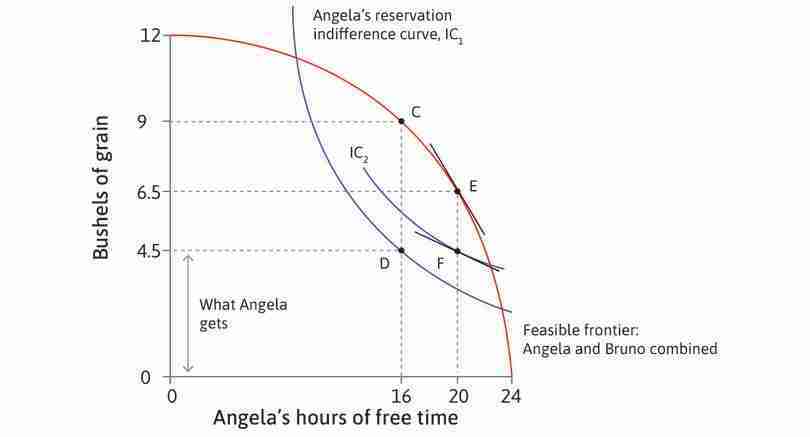
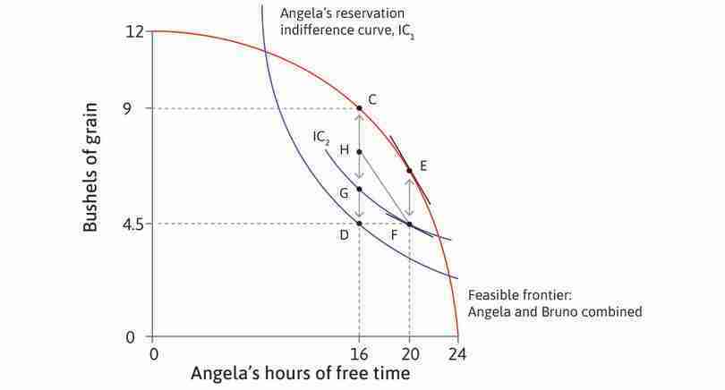
- Because you are not on the Pareto efficiency curve! Under your new law, Bruno is getting 2 bushels, and cannot make you work for more than 4 hours. So why don’t you offer to continue to pay him 2 bushels, in exchange for agreeing to let you keep anything you produce above that? Then you get to choose how many hours you work.
The small print in the law allows a longer work day if both parties agree, as long as the workers’ reservation option is a 4-hour day if no agreement is reached.
Now redraw Figure 5.11 and use the concepts of the joint surplus and the Pareto efficiency curve from Figure 5.10 to show Angela how she can get a better deal.
- You
- Look at Figure 5.12. The surplus is largest at 8 hours of work. When you work for 4 hours, the surplus is smaller, and you pay most of it to Bruno. If you increase the surplus, you can pay him the same amount and your own surplus will be bigger—so you will be better off. Follow the steps in Figure 5.12 to see how this works.
Bargaining to restore Pareto efficiency.
Figure 5.12 Bargaining to restore Pareto efficiency.
Angela can propose H
At allocation H, Bruno gets the same amount of grain—CH = EF. Angela is better off than she was at F. She works longer hours but has more than enough grain to compensate her for the loss of free time.
Figure 5.12d At allocation H, Bruno gets the same amount of grain—CH = EF. Angela is better off than she was at F. She works longer hours but has more than enough grain to compensate her for the loss of free time.
A win–win agreement by moving to an allocation between G and H
F is not Pareto efficient because MRT > MRS. If they move to a point on the Pareto efficiency curve between G and H, Angela and Bruno can both be better off.
Figure 5.12e F is not Pareto efficient because MRT > MRS. If they move to a point on the Pareto efficiency curve between G and H, Angela and Bruno can both be better off.
The move away from point D (at which Bruno had all the bargaining power and obtained all the gains from exchange) to point H where Angela is better off consists of two distinct steps:
- From D to F, the outcome is imposed by new legislation: This was definitely not win–win. Bruno lost because his economic rent at F is less than the maximum feasible rent that he got at D. Angela benefitted.
- Once at the legislated outcome, there were many win–win possibilities open to them: They are shown by the segment GH on the Pareto efficiency curve. Win–win alternatives to the allocation at F are possible by definition, because F was not Pareto efficient.
Bruno wants to negotiate. He is not happy with Angela’s proposal of H.
- Bruno
- I am no better off under this new plan than I would be if I just accepted the short-hours legislation.
- You
- But Bruno, Angela now has bargaining power, too. The legislation changed her reservation option, so it is no longer 24 hours of free time at survival rations. Her reservation option is now the legislated allocation at point F. I suggest you make her a counter offer.
- Bruno
- Angela, I’ll let you work the land for as many hours as you choose, if you pay me half a bushel more than EF.
They shake hands on the deal.
Because Angela is free to choose her work hours, subject only to paying Bruno the extra half bushel, she will work for 8 hours where MRT = MRS. Because this deal lies between G and H, it is a Pareto improvement over point F. Moreover, because it is on the Pareto-efficient curve CD, we know there are no further Pareto improvements to be made. This is true of every other allocation on GH—they differ only in the distribution of the mutual gains, as some favour Angela while others favour Bruno. Where they end up will depend on their bargaining power.
Question 5.11 Choose the correct answer(s)
In Figure 5.12, Angela and Bruno are at allocation F, where she receives 3 bushels of grain for 4 hours of work. From the figure, we can conclude that:
- Along EF, MRS < MRT. Therefore, EF is not Pareto efficient—there are other allocations where both would be better off.
- In area GHF, Angela is on a higher indifference curve than IC2, and Bruno has more grain than EF, so both are better off.
- Points on GD are Pareto efficient, but below G, Angela is on a lower indifference curve than at F, so she would be worse off.
- Points on GH are all Pareto efficient, but Bruno and Angela are not indifferent. He prefers points nearer to G, and she prefers points nearer to H.
5.8 The lessons from Angela and Bruno’s story
Angela’s farming skills and Bruno’s ownership of land provided an opportunity for mutual gains from exchange.
The same is true when people directly exchange, or buy and sell, goods for money. Suppose you have more apples than you can consume, and your neighbour has an abundance of pears. The apples are worth less to you than to your neighbour, and the pears are worth more to you. Therefore, it must be possible to achieve a Pareto improvement by exchanging some apples and pears.
When people with differing needs, property, and capacities meet, there is an opportunity to generate gains for all of them. That is why people come together in markets, online exchanges, or pirate ships. The mutual gains are what we call the surplus.
The allocations that we observe through history are largely the result of the institutions, including property rights and bargaining power, that were present in the economy. Figure 5.13 summarizes what we have learnt about the determination of economic outcomes from the succession of scenarios involving Angela and Bruno:
- Technology and biology determine whether or not they are able to mutually benefit: This is because they determine the technically feasible set of allocations in Section 5.4. If Bruno’s land had been so unproductive that Angela’s labour could not produce enough to keep her alive, then there would have been no room for a deal.
- Economically feasible allocations must be Pareto improvements of their reservation options: Those reservation options may depend on institutions (such as Angela’s survival rations from the government (Section 5.5) or legislation on working hours in Section 5.7.
- The outcome of an interaction depends both on what people want and their ability to get it: Their preferences, and the institutions that provide their bargaining power, decide how the surplus is distributed in Section 5.7.
The story of Angela and Bruno highlights that, if we have institutions under which people can jointly deliberate, agree on, and enforce alternative allocations, then it may be possible to achieve a fairer outcome that is also Pareto efficient. Angela and Bruno did this through a combination of legislation and bargaining between themselves (point H).
5.9 Measuring economic inequality
In our analysis of the interaction between Angela and Bruno, we have assessed the allocations in terms of Pareto efficiency. We have seen that they (or at least one of them) can be better off if they can negotiate a move from a Pareto-inefficient allocation to one on the Pareto efficiency curve.
Fairness and inequality
- endowment
- The facts about an individual that may affect his or her income, such as the physical wealth a person has, either land, housing, or a portfolio of shares (stocks). Also includes level and quality of schooling, special training, the computer languages in which the individual can work, work experience in internships, citizenship, whether the individual has a visa (or green card) allowing employment in a particular labour market, the nationality and gender of the individual, and even the person’s race or social class background. See also: human capital.
But the other important criterion for assessing an allocation is fairness. We know that Pareto-efficient allocations can be highly unequal. In the case of Angela and Bruno, inequality resulted directly from differences in bargaining power, but also from differences in their endowments—what they each owned before the interaction (their initial wealth). Bruno owned land, while Angela had nothing except time and the capacity to work. Differences in endowments, as well as institutions, may in turn affect bargaining power.
The Gini coefficient
In our parable, summarized in Figures 5.2 and 5.3, Angela and Bruno lived under a series of four distinct institutional settings—Angela as an independent farmer; Bruno as the enforcer with unlimited power over Angela; both living under the rule of private property and voluntary transactions, first without and later with a democratic government. In the first—Angela as an independent farmer—Bruno was not in the picture, so she could enjoy everything she produced. But in the last three, Bruno’s share of what Angela produced differed, resulting in differing levels of inequality between the two.
If we wanted to say how unequal the two were in the amount of grain they could consume, we could say that, under Bruno’s rule of force (Figure 5.7), he got 6 bushels and she got 4, so the difference in what they got—the inequality—was 2 bushels of grain. But if we wanted to compare this measure of inequality with what some other enforcer and farmer—such as a farmer growing apples—were experiencing, we would run into trouble as we would be comparing ‘apple-differences’ with ‘grain-differences’. To make the measures comparable, we could divide the difference—2 bushels of grain in the Angela and Bruno case—by the average amount of grain that each got—that is (6 + 4)/2 = 5. Our measure of inequality would be:
This would work if there were just two people in the economy, but remember we introduced the two-person model as a simplification that will help us understand economies made up of a great many people. Even in the Bruno and Angela case, this was highly unrealistic because, in most real-life cases, Bruno would have many Angelas to take advantage of, just as the landlords in West Bengal each received rent from a great many bargadars.
- Gini coefficient
- A measure of inequality of any quantity such as income or wealth, varying from a value of zero (if there is no inequality) to one (if a single individual receives all of it).
To assess inequality, economists often use a measure called the Gini coefficient, named after the Italian statistician, Corrado Gini (1884–1965). The Gini coefficient is based—like our analysis of inequality in the above Bruno and Angela example—on the differences in incomes, wealth or some other measure between people. You have already encountered (in Unit 1) the rich/poor ratio as a way of measuring inequality between the rich and the poor. The Gini coefficient has the advantage that it includes information about everyone, not just the rich and the poor, but those ‘in the middle’ too.
To see what this means, consider the three-person population shown in Figure 5.14. The circles are people and the numbers within the circles are the income received. The numbers next to the arrows are the differences between the two people, indicated by the arrows. The Gini coefficient is calculated from two pieces of information:
- The average of the differences between the people: In the example, this is (10 + 8 + 2)/3 = 20/3 = 6.67
- The average income of the people: In the example, this is (12 + 4 + 2)/3 = 6
The Gini coefficient is equal to one-half times the first number (the average difference) divided by the second number (the average income). For the example, the Gini equals 0.5(6.67/6) = 0.56. The Gini coefficient is equal to 1 if a single person owns all the income, and 0 if everyone has the same income.
- If one person has all the income: That is, 18, then the average of the differences would be (18 + 18 + 0)/3 = 12. The average income, as before, would be 6, so the Gini coefficient would be 1.
- If they all have the same income: Then there are no differences between any of the pairs, so the Gini coefficient must be zero.
Income differences among pairs of households.
Figure 5.14 Income differences among pairs of households.
In general, when we calculate the Gini coefficient, we obtain a number between 0 (perfect equality) and 1 (extreme inequality). The more unequally resources are distributed amongst the members of the population, the larger is the Gini coefficient.
Measuring inequality—the Lorenz curve
- Lorenz curve
- A graphical representation of inequality of some quantity such as wealth or income. Individuals are arranged in ascending order by how much of this quantity they have, and the cumulative share of the total is then plotted against the cumulative share of the population. For complete equality of income, for example, it would be a straight line with a slope of one. The extent to which the curve falls below this perfect equality line is a measure of inequality. See also: Gini coefficient.
A useful tool for looking at the entire distribution of income or wealth representing and comparing distributions of income or wealth across countries, is the Lorenz curve (invented in 1905 by Max Lorenz (1876–1959), an American economist, while he was still a student). It indicates how much disparity there is in income, or any other measure, across the population.3
The Lorenz curve shows the entire population lined up along the horizontal axis from the poorest to the richest. The height of the curve at any point on the horizontal axis indicates the fraction of total income received by the fraction of the population given by that point on the horizontal axis.
To see how this works, imagine a village in which there are 10 landowners, each owning 10 hectares, and 90 others who farm the land as sharecroppers, but who own no land (like Angela in the model or a bargadar in Bengal). The Lorenz curve is the blue line in Figure 5.15. Lining the population up in order of land ownership, the first 90% of the population own nothing, so the curve is flat. The remaining 10% own 10 hectares each, so the ‘curve’ rises in a straight line to reach the point where 100% of people own 100% of the land.
If each member of the population owned one hectare of land—perfect equality in land ownership—then the Lorenz curve would be a line at a 45-degree angle, indicating that the ‘poorest’ 10% of the population have 10% of the land, and so on (although in this case, everyone is equally poor and equally rich).
The Lorenz curve allows us to see how far a distribution departs from this line of perfect equality. Figure 5.16 shows the distribution of income that would have resulted from the prize-sharing system described in the articles of the pirate ship, the Royal Rover, discussed in the introduction to this unit. The Lorenz curve is very close to the 45-degree line, showing how the institutions of piracy allowed ordinary members of the crew to claim a large share of income.
In contrast, when the Royal Navy’s ships, Favourite and Active, captured the Spanish treasure ship La Hermione, the division of the spoils on the two British men-of-war ships was far less equal. The Lorenz curves show that ordinary crew members received about a quarter of the income, with the remainder going to a small number of officers and the captain. You can see that the Favourite was more unequal that the Active, with a lower share going to each crew member. By the standards of the day, pirates were unusually democratic and fair-minded in their dealings with each other.
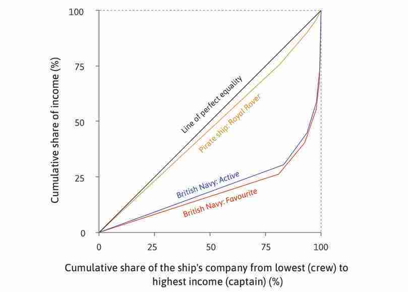
The distribution of spoils: Pirates and the Royal Navy.
Figure 5.16 The distribution of spoils: Pirates and the Royal Navy.
The Royal Rover
The Lorenz curve for the Royal Rover is very close to the line of perfect equality. Income was shared quite equally between crew members.
Figure 5.16b The Lorenz curve for the Royal Rover is very close to the line of perfect equality. Income was shared quite equally between crew members.
The British Navy ships
In contrast, the Lorenz curves for the British Navy’s ships are much further away from the line of perfect inequality. Income was concentrated in a small group of senior officers, with ordinary crew members receiving a much lower share.
Figure 5.16c In contrast, the Lorenz curves for the British Navy’s ships are much further away from the line of perfect inequality. Income was concentrated in a small group of senior officers, with ordinary crew members receiving a much lower share.
The Lorenz curve and the Gini coefficient
The Lorenz curve gives us a picture of the disparity of income across the whole population, and there is a very simple relationship between the Lorenz curve and the Gini coefficient. You can see that more unequal distributions have a greater area between the Lorenz curve and the 45-degree line. The Gini coefficient (or Gini ratio) introduced above, is calculated as the ratio of this area to the area of the whole of the triangle under the 45-degree line.
Using this new way of seeing the Gini coefficient, you can confirm (as you already learned) that, if everyone has the same income, (there is no income inequality), the Gini coefficient takes a value of 0. This is because the Lorenz curve would be the line of perfect equality itself, so there would be no area between the two. This is just as in the previous example under perfect equality there are no differences in the income of any pairs in the population.
We can calculate the Gini for land ownership in Figure 5.17a as area A, between the Lorenz curve and the perfect equality line, as a proportion of area (A + B), the triangle under the 45-degree line:
Figure 5.17b shows the Gini coefficients for each of the Lorenz curves we have drawn so far.
| Distribution | Gini |
|---|---|
| Pirate ship Royal Rover | 0.06 |
| British Navy ship Active | 0.59 |
| British Navy ship Favourite | 0.60 |
| The village with sharecroppers and landowners | 0.90 |
Comparing Gini coefficients.
Figure 5.17b Comparing Gini coefficients.
Strictly speaking, this graphical method of calculating the Gini gives only an approximation. To calculate it precisely, we need to work out the average difference in income between every pair of individuals in the population, as we did in the example at the beginning of this section. We know that the Gini is equal to 1 when a single individual receives all the income, but you can see from Figure 5.17b that the area method would give a number slightly less than 1. The area approximation is accurate only when the population is large.
Varieties of inequality
The Gini coefficient measures inequality using a single number. But not all inequalities are equal!
Sometimes, we are interested in whether a society is highly unequal because there is a small number of exceptionally rich people—everyone else being moderately well off—or, instead, there are a small number of very poor people—everyone else being better off. These two societies could have the same Gini coefficient, but we would think of them as quite different in the nature of the inequality that they experience.
In Figure 5.18, we show two societies with the same Gini coefficient. The area A/(A + B) is the same in each Lorenz curve but the distribution of income is far from identical. In the society on the left, one-half of the total income is split among 90 farmers; the 10 landowners get the remaining half. In the society shown on the right, 50 poor farmers get one-tenth of the income to split between them and the richer 50 farmers split the remaining 90%.
Exercise 5.5 Income inequality and its measurement
Write a short description comparing the life of a farmer in the two societies shown in Figure 5.18. Do the same comparison for landowners. You should assume that the total income in each society is identical. In particular, consider what the schools, political systems, workplaces, and cities might look like.
5.10 Comparing inequality across the world
- disposable income
- Income available after paying taxes and receiving transfers from the government.
To assess income inequality within a country, we can either look at total market income (all income from employment, self-employment, savings and investments), or disposable income, which better captures living standards. Disposable income is what a household can spend without borrowing money, after paying tax and receiving transfers (such as unemployment benefit and pensions) from the government.
In Unit 1, we compared inequality in the income distributions of countries using the rich/poor ratio. Lorenz curves give us a fuller picture of how distributions differ. Figure 5.20 shows the distribution of market income in the Netherlands in 2010. The Gini coefficient is 0.47, so by this measure it has greater inequality than the Royal Rover, but less than the British Navy ships.
- public policy
- A policy decided by the government. Also known as: government policy
The analysis of Figure 5.20 shows how redistributive government policies result in a more equal distribution of disposable income.
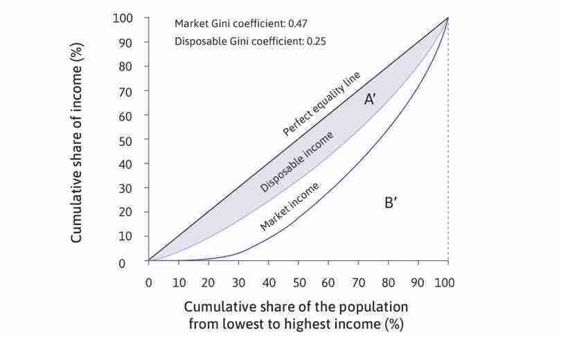
Distribution of market and disposable income in the Netherlands (2010).
Figure 5.20 Distribution of market and disposable income in the Netherlands (2010).
LIS. Cross National Data Center. Stefan Thewissen (University of Oxford) did the calculations in April 2015. Household market (labour and capital) income and disposable income are equivalized and top- and bottom-coded.

The Lorenz curve for market income
The curve indicates that the poorest 10% of the population (10 on the horizontal axis) receive only 0.1% of total income (0.1 on the vertical axis), and the lower-earning half of the population has less than 20% of the income.
Figure 5.20a The curve indicates that the poorest 10% of the population (10 on the horizontal axis) receive only 0.1% of total income (0.1 on the vertical axis), and the lower-earning half of the population has less than 20% of the income.
LIS. Cross National Data Center. Stefan Thewissen (University of Oxford) did the calculations in April 2015. Household market (labour and capital) income and disposable income are equivalized and top- and bottom-coded.
The Gini for market income
The Gini coefficient is the ratio of area A (between the market income curve and the perfect equality line) to area A + B (below the perfect equality line), which is 0.47.
Figure 5.20b The Gini coefficient is the ratio of area A (between the market income curve and the perfect equality line) to area A + B (below the perfect equality line), which is 0.47.
LIS. Cross National Data Center. Stefan Thewissen (University of Oxford) did the calculations in April 2015. Household market (labour and capital) income and disposable income are equivalized and top- and bottom-coded.
Disposable income
The amount of inequality in disposable income is much smaller than the inequality in market income. Redistributive policies have a bigger effect towards the bottom of the distribution. The poorest 10% have 4% of total disposable income.
Figure 5.20c The amount of inequality in disposable income is much smaller than the inequality in market income. Redistributive policies have a bigger effect towards the bottom of the distribution. The poorest 10% have 4% of total disposable income.
LIS. Cross National Data Center. Stefan Thewissen (University of Oxford) did the calculations in April 2015. Household market (labour and capital) income and disposable income are equivalized and top- and bottom-coded.
The Gini for disposable income
The Gini coefficient for disposable income is lower. The ratio of areas A′ (between the disposable income curve and the perfect equality line) and A′ + B′ (below the perfect equality line) is 0.25.
Figure 5.20d The Gini coefficient for disposable income is lower. The ratio of areas A′ (between the disposable income curve and the perfect equality line) and A′ + B′ (below the perfect equality line) is 0.25.
LIS. Cross National Data Center. Stefan Thewissen (University of Oxford) did the calculations in April 2015. Household market (labour and capital) income and disposable income are equivalized and top- and bottom-coded.
Notice that, in the Netherlands, almost one-fifth of the households have a near-zero market income, but most nonetheless have enough disposable income to survive, or even live comfortably—the poorest one-fifth of the population receive about 10% of all disposable income.
The Gini and the 90/10 ratio are widely used to measure income inequality, but they are not the only measure. Recall that we used the rich/poor ratio in Unit 1, which is similar but not precisely the same as the 90/10 ratio.
Figure 5.21 compares the Gini coefficients for disposable and market income across a large sample of countries, ordered from left to right, from the least to the most unequal by the disposable income measure. The main reason for the substantial differences between nations in disposable income inequality is the extent to which governments can tax well-off families and transfer the proceeds to the less well off.
Notice that:
- The differences between countries in disposable income inequality (the top of the lower bars) are much greater than the differences in inequality of market incomes (the top of the upper bars).
- The US and the UK are among the most unequal of the high-income economies.
- The few poor and middle-income countries for which data is available are even more unequal in disposable income than the US, but …
- … (with the exception of South Africa) this is mainly the result of the limited degree of redistribution from rich to poor, rather than unusually high inequality in market income.
Income inequality in market and disposable income across the world.
Figure 5.21 Income inequality in market and disposable income across the world.
LIS. Cross National Data Center. Stefan Thewissen (University of Oxford) did the calculations in April 2015.
Two important questions arise from the figure—why is market income inequality so different between, say South Africa and South Korea? And, why do we see such a big difference in market income inequality and disposable income inequality—one measure of how much rich–to-poor redistribution the government does? You can see this by comparing China, India, and the US, on the one hand, with Sweden, Germany, and Hungary, on the other.

Because the Gini coefficient uses a single number to measure how unequal people are according to some economic indicator such as their income, it allows very intuitive statements about what this number means.
If we were to compare every possible pair in the population, the richer of the pair will have some multiple of the income or wealth of the poorer given by the following equation:
So, if the Gini coefficient was 0.5, then the richer person is, on average, three times richer than the poorer person (1.5/0.5 = 3). This corresponds to the rich person getting three-quarters of the pie and the poorer person getting one-quarter.
Applying this to the Dutch income distribution, this means that if you randomly selected many pairs of people from the Dutch population on average the richer of the two would be (1 + 0.47)/(1 – 0.47) = 2.78 times as rich as the poorer.
The disposable income Gini coefficient of 0.25 means that on average the richer of the pairs randomly selected in a population will have 1.67 times the disposable income of the poorer (the ratio for market incomes was 2.78).
Exercise 5.6 Comparing distributions of wealth
Figure 5.22 shows three alternative distributions of land ownership in a village with 100 people and 100 hectares of land. Draw the Lorenz curves for each case.
For cases I and III, calculate the Gini. For case II, show on the Lorenz curve diagram how the Gini coefficient can be calculated.
Exercise 5.7 Using Excel: Inequalities among your classmates
- Record the heights of you and your classmates in an Excel spreadsheet. Now, make a table with percentiles (0–100, in increments of 1) in one column and the corresponding cumulative share of the population in another column. Use this table to draw a Lorenz curve for height. Follow the walk-through in Figure 5.23 on how to draw a Lorenz curve in Excel.
Drawing a Lorenz curve.
Figure 5.23 Drawing a Lorenz curve.
The data
We will be drawing a Lorenz curve of the height data in Column A (30 observations total, height measured in centimetres).
Figure 5.23a We will be drawing a Lorenz curve of the height data in Column A (30 observations total, height measured in centimetres).
Calculate the heights corresponding to each decile
First, we will make a table with columns that correspond to the horizontal and vertical axis of the Lorenz curve diagram (Columns C and E respectively). We need Column D to calculate the values in Column E.
Figure 5.23b First, we will make a table with columns that correspond to the horizontal and vertical axis of the Lorenz curve diagram (Columns C and E respectively). We need Column D to calculate the values in Column E.
Calculate the cumulative share of height ‘owned’ by each decile
To calculate the values in Column E, we need to add up all the heights with values less than the corresponding value in Column D, and then divide by the sum of all heights in Column A.
Figure 5.23c To calculate the values in Column E, we need to add up all the heights with values less than the corresponding value in Column D, and then divide by the sum of all heights in Column A.
Calculate the cumulative share of height ‘owned’ by each decile
The ‘$’ signs in the formula shown ensure that the same range of cells is used, even when copying the formula to other cells. Without this sign, Excel would use a different range for each cell (e.g. the cell below would have A3:A32).
Figure 5.23d The ‘$’ signs in the formula shown ensure that the same range of cells is used, even when copying the formula to other cells. Without this sign, Excel would use a different range for each cell (e.g. the cell below would have A3:A32).
Draw a Lorenz curve (line chart)
After step 8, the line chart will look like the chart on the left above. The Lorenz curve is in orange, and the perfect equality line is in blue. The Gini coefficient is 5.79, indicating near perfect equality.
Figure 5.23e After step 8, the line chart will look like the chart on the left above. The Lorenz curve is in orange, and the perfect equality line is in blue. The Gini coefficient is 5.79, indicating near perfect equality.
Another Lorenz curve
Our curve looks similar to the Lorenz curve from the Gini coefficient calculator website, shown here.
Figure 5.23f Our curve looks similar to the Lorenz curve from the Gini coefficient calculator website, shown here.
- Using a Gini coefficient calculator, calculate the degree of inequality of height (in cm) among your classmates. Check that your Lorenz curve looks like the one shown.
- Explain any differences between the Gini coefficient you calculated for height, and those for market and disposable income in Figure 5.21.
Question 5.12 Choose the correct answer(s)
Based on Figure 5.20, which of the following statements are true?
- This is true from the Lorenz curve for market income.
- The income distribution is more unequal for market income than for disposable income. Therefore, the Gini coefficient is larger for market income.
- Disposable income is defined as market income minus tax plus cash transfers.
- The Lorenz curve for disposable income suggests that the poorest one-fifth of the population receive about 10% of all disposable income.
Question 5.13 Choose the correct answer(s)
Based on Figure 5.21, which of the following statements are true?
- As the Gini coefficient is a measure of income inequality, a lower coefficient implies that the incomes are more equally distributed.
- More effective redistributive policies would result in a larger difference between market income and disposable income Gini coefficients.
- The differences between the height of the blue bars is smaller than that of the red bars.
- In most cases, redistributive policies help reduce inequality in disposable income, so that countries with a higher degree of market income inequality do not necessarily have a higher degree of disposable income inequality (for example, Ireland and Hungary).
Find out more The Gini coefficient as a measure of inequality
There are two other ways of looking at the Gini coefficient that will help you understand what the number means.
First, from the example in Figure 5.14, if the richest person had an income of 10, then the average difference between all pairs divided by the mean income in the population would be twice the Gini coefficient. So, in this particular example where the Gini coefficient is 0.5, the average difference is the mean income itself. You can try another example for yourself by altering the numbers in the diagram in Figure 5.14.
Second, suppose there are just two people in a population and they are dividing a ‘pie’ representing total wealth. The portion received by the disadvantaged person is simply one-half of (1 − Gini). So in the example above where the Gini is 0.5, the poorer person gets a slice equal to one-quarter of the pie and the richer person gets three-quarters of the pie.
For another interpretation of the Gini coefficient, see Einstein 19.1 in The Economy.
How Operation Barga changed the Lorenz curve and the Gini coefficient
Angela and Bruno live in the hypothetical world of an economic model, but real farmers and landowners face similar problems.
We do not have detailed information on the change in inequality that accompanied the implementation of Operation Barga described in Section 5.1, but we can illustrate the effect of the land reform on the distribution of income in the hypothetical village of the previous section, with 90 sharecroppers and 10 landowners. Figure 5.24 shows the Lorenz curves. Initially, the farmers pay a rent of 50% of their crop to the landowners. Operation Barga raises the farmer’s crop share to 75%, moving the Lorenz curve towards the 45-degree line. As a result, the Gini coefficient of income is reduced from 0.4 (similar to the US) to 0.15 (well below that of the most equal of the rich economies, such as Denmark). The ‘Find out more’ box at the end of this section shows you how the Gini coefficient depends on the proportion of farmers and their crop share.
Find out more The Lorenz curve and the Gini coefficient in a class-divided economy with a large population
Think about a population of 100 people in which a fraction, n, produces the output, and the others are employers (or landlords, or other claimants on income who are not producers).
Take, as an example, the farmers and landlords in the text (in West Bengal). Each of the n × 100 farmers produces q and they each receive a fraction, s, of this; so each of the farmers has income sq. The (1 − n) × 100 employers each receive an income of (1 − s)q.
Figure 5.25 presents the Lorenz curve and the perfect equality line, similar to Figure 5.24 in the text.
The slope of the line separating area A from B1 is s/n (the fraction of total output that each farmer gets), and the slope of the line separating area A from B3 is (1 − s)/(1 − n), the fraction of total output that each landlord gets. We can approximate the Gini coefficient by the expression A/(A + B), where in the figure B = B1 + B2 + B3.
We can express the Gini coefficient in terms of the triangles and rectangle in the figure. To see how, note that the area of the entire square is 1, while the area (A+B) under the perfect equality line is 1/2. The area A is (1/2) − B. Then we can write the Gini coefficient as:
We can see from the figure that:
So
This means that the Gini coefficient in this simple case is just the fraction of the total population producing the output (the farmers) minus the fraction of the output that they receive in income.
Inequality will increase in this model economy if:
- The fraction of producers in the economy increases but the total share of output they receive remains unchanged: This would be the case if some of the landlords became farmer tenants, each receiving a fraction, s, of the crop they produced.
- The fraction of the crop received by the producers falls.
5.11 Conclusion
Figure 5.13 showed the fundamental determinants of economic outcomes.
Figure 5.13 showed the fundamental determinants of economic outcomes.
Interactions among people are governed by political and economic institutions, which are the rules of the game in a society. Institutions comprise both formal rules (like laws and regulations) and informal customs (such as social norms), as well as the methods by which these are enforced.
The economic rent gained by each party to an interaction is how much better off they are with the interaction than they would have been without it, at their reservation option. When people voluntarily engage in an interaction, there must be economic rents. The sum of economic rents is the joint surplus.
Two important aspects of any interaction are the size of the joint surplus and how it is distributed among the parties. The latter depends on their bargaining power, which is influenced by institutions (such as property rights or how the government is selected) and conditions affecting the extent to which people cooperate rather than act individually.
In a democracy, government policies can increase the fairness of how the joint surplus is shared. An example studied is Operation Barga in India. Both government policies and private bargaining can implement a more efficient allocation.
We have used our constrained choice model toolkit to show that even the very powerful face limits as to how much they can get. The same model allows us to analyse how different institutional settings affect the degree of inequality in resulting allocations, by altering the balance of bargaining power between the parties engaging in the exchange.
While technology (the production function) determines the feasible frontier, subsistence requirements impose biological constraints. Together, these form the boundaries of the technically feasible set. With voluntary interactions under the rule of law rather than the rule of force, individuals’ reservation indifference curves are a more binding constraint, defining the economically feasible set.
If (and only if) for some allocation, the MRS (slope of indifference curve—the trade-off between objectives) is equal to the MRT (slope of feasible frontier—the trade-off in what is feasible), then the allocation is Pareto efficient. The set of all Pareto-efficient allocations is the Pareto efficiency curve.
The Gini coefficient is a measure of inequality based on differences in income, wealth, or some other economic indicator among all the members of an economy. The difference between the market income Gini and the disposable income Gini measures how taxes and transfers contribute to the redistributive effects of government policies in that country. The Lorenz curve gives us a picture of the disparity of income across the entire population and allows us to see that the nature of inequality may differ, even in countries with the same Gini coefficient.
5.12 Doing Economics: Measuring inequality: Lorenz curves and Gini coefficients
To get hands-on experience constructing different measures of inequality and using a variety of data sources, go to Doing Economics Empirical Project 5. In this project, you will learn how to construct Gini coefficients and Lorenz curves from raw data. By constructing other measures of income inequality, the project shows how a country’s income distribution can be summarized. A policymaker may wish to know how a proposed policy affects inequality as measured by these different summary indicators.
The project looks at how gender inequality can be measured and at how inequality can be accounted for in indices of wellbeing such as the Human Development Index.
Learning objectives
In this project you will:
- draw Lorenz curves and interpret the Gini coefficient
- calculate and interpret alternative measures of income inequality
- research other dimensions of inequality and how they are measured.
5.13 References
- Banerjee, Abhijit V., Paul J. Gertler, and Maitreesh Ghatak. 2002. ‘Empowerment and Efficiency: Tenancy Reform in West Bengal’. Journal of Political Economy 110 (2): pp. 239–80.
- Leeson, Peter T. 2007. ‘An-arrgh-chy: The Law and Economics of Pirate Organizations’. Journal of Political Economy 115 (6): pp. 1049–94.
- Lorenz, Max O. 1905. ‘Methods of Measuring the Concentration of Wealth’. Publications of the American Statistical Association 9 (70).
- Raychaudhuri, Ajitava. 2004. Lessons from the Land Reform Movement in West Bengal, India. Washington, DC: World Bank.
-
Abhijit V. Banerjee, Paul J. Gertler, and Maitreesh Ghatak. 2002. ‘Empowerment and Efficiency: Tenancy Reform in West Bengal’. Journal of Political Economy 110 (2): pp. 239–80. ↩
-
Ajitava Raychaudhuri. 2004. Lessons from the Land Reform Movement in West Bengal, India. Washington, DC: World Bank. ↩
-
Max O. Lorenz. 1905. ‘Methods of Measuring the Concentration of Wealth’. Publications of the American Statistical Association 9 (70). ↩
