3 Public policy for fairness and efficiency
3.1 Introduction
- Public policies are evaluated on the basis of whether their intended outcomes are efficient and fair, and whether they can be implemented.
- People may consider an outcome to be unfair, either because who gets what is thought to be unjust, or because the rules of the game determining this distribution are seen as unfair.
- Experiments with a new game, the ultimatum game, show that people care about fairness, are willing to sacrifice their own material payoffs to avoid unfair outcomes, and are willing to punish unfair behaviour in others.
- Successful public policies such as taxes and subsidies change the circumstances in which people decide how to act, and in so doing create a new allocation that will not be sustained unless it is a Nash equilibrium.
- Understanding people’s responses to policies so that we can better understand the likely outcomes of our policy choices is a major challenge for economists and policymakers.
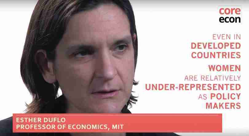
In most countries and throughout human history, women have been underrepresented in positions of political leadership. We can argue that this affects the public policies that governments create. For example, countries in which women are more equally represented as members of parliament or heads of state have spent more to support the less well off.
But the fact that there are pro-poor policies when women are in powerful positions—as in Norway, Sweden, and the other Nordic countries—does not mean that electing women has caused these policies. It could be that countries that have values that lead them to support pro-poor policies are also more likely to elect women. In this case, they would enact the same pro-poor policies, even if women were not elected.
This raises the difficult problem of causation, introduced in Section 1.8, where we compared economic growth under capitalist West Germany and centrally planned East Germany. The data in Figure 1.15 indicated that the difference in their economic institutions was probably a cause (not just a correlate) of the divergent economic fortunes of the two Germanies. Economists are interested in what causes what, because we would like economic knowledge to be useful. One way it can be useful is if it contributes to the design of policies that would cause better outcomes to happen.
A study of changes in women’s voting rights in the US, and the changes in public policy that followed, provides a similar opportunity to identify whether increased political power for women actually caused changes in policies. The US is a particularly useful laboratory for this kind of study because voting laws differ by state. As a result, women gained the right to vote at different times, starting in 1869 in Wyoming. In 1920, the Nineteenth Amendment to the US Constitution granted the vote to women in all of the remaining states that had not yet granted this right.
Grant Miller, an economist, has used the date at which women got the right to vote to do a before-and-after comparison of the actions taken by elected officials, public expenditures related to child health, and health outcomes for children.1
Miller chose to focus on child healthcare policies because women had campaigned to expand health services for children. It is therefore reasonable to assume that women would have chosen different policies at this time than men would have chosen. During the nineteenth century and before, however, those who argued that only men should vote often claimed that women were represented through their husbands, brothers, and fathers.
- natural experiment
- An empirical study exploiting naturally occurring statistical controls in which researchers do not have the ability to assign participants to treatment and control groups, as is the case in conventional experiments. Instead, differences in law, policy, weather, or other events can offer the opportunity to analyse populations as if they had been part of an experiment. The validity of such studies depends on the premise that the assignment of subjects to the naturally occurring treatment and control groups can be plausibly argued to be random.
Miller’s study is a ‘natural experiment’, and is similar to the case of the two Germanies:
- It is an experiment: The variable that interests us—the right to vote for women—was the only difference likely to affect public spending and child health. Other things that might have had an effect—the state’s tax base, or improvements in medical knowledge, for example—are held constant by looking at the same state at roughly the same time, and at changes occurring in other states in which women did not have the right to vote.
- It is natural: It was not designed or conducted in a lab, but happened in the course of history.
The logic of a natural experiment is illustrated in this diagram, in which each arrow represents possible causes that Miller explored.

Women get the vote: flowchart
Miller’s research asked two questions: ‘Did women’s voting rights have a causal effect on what the government did?’ (the first arrow), and ‘Did the changes in government programs have any causal effect on children’s wellbeing?’ (the second arrow).
- difference-in-difference
- A method that applies an experimental research design to outcomes observed in a natural experiment. It involves comparing the difference in the average outcomes of two groups, a treatment and control group, both before and after the treatment took place.
- causality
- A direction from cause to effect, establishing that a change in one variable produces a change in another. While a correlation is simply an assessment that two things have moved together, causation implies a mechanism accounting for the association, and is therefore a more restrictive concept. See also: natural experiment, correlation.
To explore whether women’s voting rights were a cause of the changes in spending and improved child health, Miller adopted what is called a ‘difference-in-difference’ method. To identify the first arrow above as a causal relationship rather than just a correlation, he compared the difference in spending before and after the change in voting rights in the states in which this occurred, with changes in spending over the same period, but in states in which there was no change in voting rights.
If the difference was greater in the states where women had gained voting rights, he could conclude that the change in voting rights had caused the differences in spending.
The key assumption for the difference-in-difference method is that any relevant changes that took place in the state of Wyoming between 1868 and 1870 (when women were granted the vote), except the change in women’s voting rights itself, were common to other states that did not grant women the right to vote during those years.
Here is what Miller found:
- Social services increased: Looking state-by-state at the date women got the right to vote, enfranchisement boosted social service spending by 24%. It had no apparent effect on public spending in other areas.
- Spending on children increased: Within a year of the passage of the Nineteenth Amendment, the US Congress voted for a substantial increase in public health spending aimed at children. A historian concluded that ‘the principal force moving Congress was fear of being punished at the polls … by women voters.’
- Child deaths decreased: In 1900, one in five children in the US did not live to the age of five. The deaths of children under the age of nine fell by between 8% and 15%. This was primarily as a result of the public programs that had been adopted, especially large-scale door-to-door hygiene campaigns.
Healthcare programs, based on the recent revolution in scientific knowledge of bacteria and disease, prevented an estimated 20,000 child deaths per year. Votes for women helped to achieve this.
In many countries today, women participate much less in political life and leadership than do men, and political systems are often less responsive to the needs of women than men. But if we want to show that it makes a difference when women gain more political power, we must always distinguish, as Miller did, between causes and correlations.
India has provided an unusual laboratory to do this. In our ‘Economist in action’ video, Esther Duflo explains what happened when the government of India mandated that randomly selected villages elect a woman to head their local council.
The video shows that reserving positions for women to head village councils:
- increased public spending on the public services that women preferred, like wells
- reduced receipts of bribes by those in power
- transformed stereotypes, so that men in villages with women leaders perceived them more as leaders, rather than solely in domestic roles.
The reduction in child mortality in the US, and the changes in village council policies in India, illustrate the capacity of governments to provide solutions to problems arising in the economy.
In the US, for example, many children, particularly in poor families, no longer died from readily preventable diseases. The policies also limited the spread of communicable diseases among all members of the population.
In this case, the government provided a public good—better sanitation and public information about hygiene—that improved conditions for most Americans, and specially helped the least well off. These two objectives—promoting gains for all and correcting unfairness—are foremost among the standards by which we evaluate economic outcomes and policies to improve them.
Question 3.1 Choose the correct answer(s)
According to the ‘Economist in action’ video featuring Esther Duflo:
- The villages that had to increase female representation in their council were essentially chosen by lottery, so we can reasonably conclude that any changes in policymaking are due to greater women representation and not due to other characteristics of the village or village council.
- Rather than asking villagers directly, Duflo had them listen to the same policy speech read by either a male or a female, and asked them to rank which speech they preferred.
- This is a long-term effect of the local council reform.
- After exposure to women policymakers, girls’ aspirations increased and they were less likely to drop out of middle school.
3.2 Goals of public policy
- public policy
- A policy decided by the government. Also known as: government policy
To illustrate these two objectives of public policy—promoting gains for all and correcting unfairness—we return to the problem of free riding, as illustrated by the tragedy of the commons introduced in the previous unit. Let’s explore how public policy might avert the tragedy.
Here is how the tragedy of the commons unfolds, according to its author, Garrett Hardin:2
Picture a pasture open to all. … each herdsman … seeks to maximize his gain … [and] will try to keep as many cattle as possible on the commons. … he asks, ‘What is the utility to me of adding one more animal …?’ 1) The positive component … the herdsman receives all of the proceeds from the sale of the additional animal. 2) The negative component … the effects of overgrazing are shared by all of the herdsman [so] the negative utility for any decision-making herdsman is only a fraction of the total [negative effect].
The tragedy seems inevitable:
The only sensible course for him to pursue is to add another animal to his herd. And another. But this is the conclusion reached by each and every … herdsman sharing a commons. Therein is the tragedy. Ruin is the destination towards which all men rush, each pursuing his own best interest. Freedom in the commons brings ruin to all.
Now think about how government policy might improve the situation.
Cows as common property
A policymaker might reason, as Hardin did, that the problem is that all herders have access to the pasture and they make their decisions independently—without taking account of the negative external effect on the other herders if they decide to put additional cows on the pasture. This suggests a solution. If they owned all of the cows jointly, they could decide together how many of them to put on the pasture. That way, there would be no external effects of placing too many cows on the pasture. The costs of overgrazing would be experienced by all members of the decision-making body.
If they owned the cows jointly, they would take care of the pasture. But, under this arrangement the cows would now be owned by everyone. So who would take care of the cows? Each of the herders would have an incentive to free ride on the others by letting somebody else tend the cattle. The tragedy of the commons has become the tragedy of the cows!
Private property averts the tragedy
Our policymaker might try a different approach. If one herder was given access to the pasture and the rest excluded, then this lucky herder would reason in a different way—‘If I put an additional cow on the pasture, this gives me one more cow, but less pasture for the rest of my own cows. So, I should limit the size of my herd.’
The tragedy has been averted. Converting the pasture to the private property of the one lucky herder addresses the root of the problem, which was that each herder did not consider the effects of a decision on the other herders. Now there is only one herder, and they will take account of the damage that overgrazing might inflict on the pasture and the cattle on it.
Is this a fair allocation?
What about the herders who have been excluded from the pasture? Denying them access to the pasture hardly seems fair. An unfair outcome may not be sustainable in the long run, even if it provided an efficient solution to the initial problem.
Whether it is fishermen seeking to make a living while not depleting the fish stocks, or farmers maintaining the channels of an irrigation system, herders overgrazing a pasture, or two people dividing up a pie, we want to be able to both describe what happens and evaluate it—is it better or worse than other potential outcomes? The first involves facts; the second involves values.
- allocation
- A description of who does what, the consequences of their actions, and who gets what as a result (for example in a game, the strategies adopted by each player and their resulting payoffs).
We call the outcome of an economic interaction an allocation. Taking as an example the climate change game described in Unit 2, each of the four outcomes and the resulting payoffs for the two players, the US and China, is called an allocation.
Our discussion of the tragedy of the commons has evaluated outcomes along two dimensions: ruining the pasture was not a sensible way to use the resource, but averting the tragedy by assigning the property right to the pasture to a single herder did not seem fair. We will illustrate these two objectives—which we will call efficiency and fairness—by a new kind of social interaction, which we call the ultimatum game. After we have played this game, we will explain these important terms in more detail.
3.3 Fairness and efficiency in the ultimatum game
- ultimatum game
- An interaction in which the first player proposes a division of a ‘pie’ with the second player, who may either accept, in which case they each get the division proposed by the first person, or reject the offer, in which case both players receive nothing.
To study how the objectives of efficiency and fairness interact—sometimes in mutually supportive ways, but often in conflict—we turn to a new game, called the ultimatum game. It has been used around the world with experimental subjects including students, farmers, warehouse workers, and hunter-gatherers.
The subjects of the experiment play a game in which they will win some money. How much they win will depend on how they and the others in the game play. So, like the public goods game experiments in Unit 2, it is a strategic interaction in which the payoffs of each depend on the actions of the others.
Real money is at stake in experimental games like these, otherwise we could not be sure the subjects’ answers to a hypothetical question would reflect their actions in real life.
The rules of the game are explained to the players.
- They are randomly matched in pairs.
- One player is randomly assigned as the Proposer and the other the Responder.
- The subjects do not know each other, but they know the other player was recruited to the experiment in the same way.
- Subjects remain anonymous.
The Proposer is provisionally given an amount of money, say $100, by the experimenter, and instructed to offer the Responder part of it. Any split is permitted, including keeping it all, or giving it all away. We will call this amount the ‘pie’ because the point of the experiment is how it will be divided up.
The split takes the form ‘x for me, y for you’, where x + y = $100.
- The Responder knows that the Proposer has $100 to split.
- After observing the offer, the Responder accepts or rejects it.
- If the offer is rejected, both individuals get nothing.
- If it is accepted, the split is implemented—the Proposer gets x and the Responder y.
For example, if the Proposer offers $35 and the Responder accepts, the Proposer gets $65 and the Responder gets $35. If the Responder rejects the offer, they both get nothing.
This is called a take-it-or-leave-it offer. It is the ultimatum in the game’s name. The Responder is faced with a choice—accept $35 and let the other get $65, or get nothing and deprive the other player of any payoffs too.
A game tree
We start by thinking about a simplified case of the ultimatum game, represented in Figure 3.1 in a diagram called a game tree. The Proposer’s choices are either the ‘fair offer’ of an equal split, or the ‘unfair offer’ of 20 (keeping 80 for herself). Then the Responder has the choice to accept or reject. The payoffs are shown in the last row. In the actual experiments, Proposers were not confined to these two fair and unfair options. Instead, they could choose any split they wished, including proposing to give everything or nothing to the other.
Game tree for the ultimatum game in which the only choices open to the Proposer are an even split, or to keep 80 while giving 20 to the Responder.
Figure 3.1 Game tree for the ultimatum game in which the only choices open to the Proposer are an even split, or to keep 80 while giving 20 to the Responder.
- sequential game
- A game in which all players do not choose their strategies at the same time, and players that choose later can see the strategies already chosen by the other players, for example the ultimatum game. See also: simultaneous game.
The game tree is a useful way to represent social interactions because it clarifies who does what, when they choose, and the results. We see that in the ultimatum game one player (the Proposer) chooses her strategy first, followed by the Responder. This is called a sequential game because each player knows the actions of the previous player before acting (unlike the prisoners’ dilemma, for example).
A strategic interaction
What the Proposer will get depends on what the Responder does, so the Proposer has to think about the likely response of the other player. This is why it is called a strategic interaction. If you’re the Proposer you can’t try out a low offer to see what happens. You have only one chance to make an offer. How would you think this through if you were the Proposer?
- Put yourself in the place of the Responder in this game: Would you accept (50, 50)? Would you accept (80, 20)?
- Now switch roles and suppose that you are the Proposer: What split would you offer to the Responder? Would your answer depend on whether the other person was a friend, a stranger, a person in need, or a competitor?
We have some clues about how to answer these questions. Dividing something of value in equal shares (the 50–50 rule) is a social norm in many communities, as is giving gifts on birthdays to close family members and friends. Social norms are common to an entire group of people (almost all follow them) and tell a person what they should do in the eyes of most people in the community.
A Responder who thinks that the Proposer’s offer has violated a social norm of fairness, or that the offer is insultingly low for some other reason, might be willing to sacrifice their own payoff to punish the Proposer.
Exercise 3.1 Acceptable offers
Look again at the ultimatum game shown in Figure 3.1.
- Suppose the Proposer received the $100 through some other means rather than being given $100 by the experimenter: For example, she might have found it on the street, won it in the lottery, received it as an inheritance, or earned it through hard work. How might the Responder’s perception of the ($80, $20) offer depend on the way that the Proposer acquired the $100?
- Suppose that the Proposer can offer more than $50 to the Responder, and the social norm in this society is 50–50: Can you imagine anyone offering more than $50 in such a society? Why, or why not?
The problem of fairness and efficiency
If in the ultimatum game you were a Responder who cared only about your own payoffs, you would accept any positive offer, because something is better than nothing. But if you cared about fairness too, and the Proposer made you a very low offer that you considered to be unfair, you might decide to reject the offer. Neither you nor the Proposer would receive anything. This outcome—throwing away money!—cannot be efficient.
One way of eliminating this inefficiency would be to change the rules of the game so that a Responder, even one who cared very much about fairness, could not reject any offer. For obvious reasons, this is called the dictator game! There would never be money left on the table, but much like excluding all but one herder from using the pasture (in the tragedy of the commons), it would hardly be called fair.
People value fairness in practice
In a world composed only of self-interested individuals, in which everyone knew for sure that everyone else was self-interested, the Proposer would anticipate that the Responder would accept any offer greater than zero and, for that reason, would offer the minimum possible positive amount—one cent—knowing it would be accepted.
Does this prediction match the experimental data? No, it does not. As in the prisoners’ dilemma studied in the previous unit, we don’t see the outcome we would predict if people were entirely self-interested. One-cent offers get rejected. If it costs you just one cent to punish a selfish person—sending them away with nothing—it’s not difficult to see why most people are happy to do so!
Let’s see how Kenyan farmers and US students actually played the ultimatum game.
Look at Figure 3.2. Before playing the game, the researchers—a team of anthropologists and economists who conducted the same experiments throughout the world—asked their subjects to indicate (confidentially) the offers they would accept and which they would reject. The height of each bar indicates the fraction of Responders who were willing to accept the offer indicated on the horizontal axis. Offers of more than half of the pie were acceptable to all of the subjects in both countries, as one would expect.
Adapted from Joseph Henrich, Richard McElreath, Abigail Barr, Jean Ensminger, Clark Barrett, Alexander Bolyanatz, Juan Camilo Cardenas, Michael Gurven, Edwins Gwako, Natalie Henrich, Carolyn Lesorogol, Frank Marlowe, David Tracer, and John Ziker. 2006. ‘Costly Punishment Across Human Societies’. Science 312 (5781): pp. 1767–70.
Notice that the Kenyan farmers are very unwilling to accept low offers, presumably regarding them as unfair, while the US students are much more willing to do so. For example, virtually all (90%) of the farmers would say no to an offer of one-fifth of the pie (the Proposer keeping 80%), while 63% of the students would accept such a low offer. More than half of the students would accept just 10% of the pie, but almost none of the farmers would.
Although the results in Figure 3.2 indicate that attitudes differ about the importance of fairness and what constitutes fairness, nobody in the Kenyan and US experiments was willing to accept an offer of zero, even though by rejecting it they would also receive zero.
Figure 3.3 shows another way of looking at these results. The full height of each bar in Figure 3.3 indicates the percentage of the Kenyan and American Proposers who made the offer shown on the horizontal axis when they actually played the game. For example, half of the farmers made proposals of 40%. Another 10% offered an even split. Only 11% of the students made such generous offers.
Actual offers and expected rejections in the ultimatum game.
Figure 3.3 Actual offers and expected rejections in the ultimatum game.
Adapted from Joseph Henrich, Richard McElreath, Abigail Barr, Jean Ensminger, Clark Barrett, Alexander Bolyanatz, Juan Camilo Cardenas, Michael Gurven, Edwins Gwako, Natalie Henrich, Carolyn Lesorogol, Frank Marlowe, David Tracer, and John Ziker. 2006. ‘Costly Punishment Across Human Societies’. Science 312 (5781): pp. 1767–70.
What do the bars show?
The full height of each bar in the figure indicates the percentage of the Kenyan and American Proposers who made the offer shown on the horizontal axis.
Figure 3.3a The full height of each bar in the figure indicates the percentage of the Kenyan and American Proposers who made the offer shown on the horizontal axis.
Adapted from Joseph Henrich, Richard McElreath, Abigail Barr, Jean Ensminger, Clark Barrett, Alexander Bolyanatz, Juan Camilo Cardenas, Michael Gurven, Edwins Gwako, Natalie Henrich, Carolyn Lesorogol, Frank Marlowe, David Tracer, and John Ziker. 2006. ‘Costly Punishment Across Human Societies’. Science 312 (5781): pp. 1767–70.
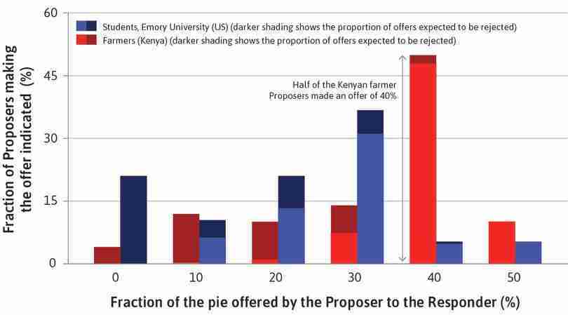
Reading the figure
For example, for Kenyan farmers, 50% on the vertical axis and 40% on the horizontal axis means half of the Kenyan Proposers made an offer of 40%.
Figure 3.3b For example, for Kenyan farmers, 50% on the vertical axis and 40% on the horizontal axis means half of the Kenyan Proposers made an offer of 40%.
Adapted from Joseph Henrich, Richard McElreath, Abigail Barr, Jean Ensminger, Clark Barrett, Alexander Bolyanatz, Juan Camilo Cardenas, Michael Gurven, Edwins Gwako, Natalie Henrich, Carolyn Lesorogol, Frank Marlowe, David Tracer, and John Ziker. 2006. ‘Costly Punishment Across Human Societies’. Science 312 (5781): pp. 1767–70.
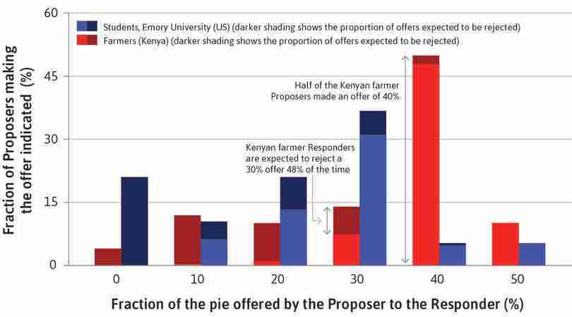
The dark-shaded area shows rejections
If Kenyan farmers made an offer of 30%, almost half of Responders would reject it. (The dark part of the bar is almost as big as the light part.)
Figure 3.3c If Kenyan farmers made an offer of 30%, almost half of Responders would reject it. (The dark part of the bar is almost as big as the light part.)
Adapted from Joseph Henrich, Richard McElreath, Abigail Barr, Jean Ensminger, Clark Barrett, Alexander Bolyanatz, Juan Camilo Cardenas, Michael Gurven, Edwins Gwako, Natalie Henrich, Carolyn Lesorogol, Frank Marlowe, David Tracer, and John Ziker. 2006. ‘Costly Punishment Across Human Societies’. Science 312 (5781): pp. 1767–70.
Better offers, fewer rejections
The relative size of the dark area is smaller for better offers. For example, Kenyan farmer Responders rejected a 40% offer only 4% of the time.
Figure 3.3d The relative size of the dark area is smaller for better offers. For example, Kenyan farmer Responders rejected a 40% offer only 4% of the time.
Adapted from Joseph Henrich, Richard McElreath, Abigail Barr, Jean Ensminger, Clark Barrett, Alexander Bolyanatz, Juan Camilo Cardenas, Michael Gurven, Edwins Gwako, Natalie Henrich, Carolyn Lesorogol, Frank Marlowe, David Tracer, and John Ziker. 2006. ‘Costly Punishment Across Human Societies’. Science 312 (5781): pp. 1767–70.
The Proposer’s reasoning
But were the farmers really being generous? To answer, you should think not only about how much they were offering, but also what they must have reasoned when considering whether the Responder would accept the offer. If you look at Figure 3.3 and concentrate on the Kenyan farmers, you will see that very few proposed to keep the entire pie by offering zero (4% of them as shown in the far left-hand bar). This is no surprise, given that they must have reasoned that all of those offers would be rejected (the entire bar is dark).
On the other hand, looking at the far right of the figure, we see that for the farmers, making an offer of half the pie ensured an acceptance rate of 100% (the entire bar is light). Those who offered 30% were about equally likely to see their offer rejected as accepted (the dark part of the bar is nearly as big as the light part).
A Proposer who wanted to earn as much as possible would choose something between the extremes of trying to take it all, or dividing it equally. The farmers who offered 40% were very likely to see their offer accepted and receive 60% of the pie. In the experiment, half of the farmers chose an offer of 40%. This offer was rejected only 4% of the time, as can be seen from the tiny dark-shaded top part of the bar at the 40% offer in Figure 3.3.
Now suppose you are a Kenyan farmer and all you care about is your own payoff. Offering to give the Responder nothing is out of the question because that will ensure that you get nothing when they reject your offer. Offering half will get you half for sure—because the Responder will surely accept. But you suspect that you can do better. Something more than nothing but less than half would be your best bet. Given how likely the farmers were to reject low offers, you would maximize your payoffs on average if you offered 40%—this was the most common offer among Kenyan Proposers.
Similar calculations indicate that, among the students, the expected payoff-maximizing offer was 30%, and this was the most common offer among them. The students’ lower offers could be because they correctly anticipated that lowball offers (even as low as 10%) would sometimes be accepted. They may have been trying to maximize their payoffs and hoping that they could get away with making low offers.
How do the two populations differ? Although many of the farmers and the students offered an amount that would maximize their expected payoffs, the similarity ends there. The Kenyan farmers were more likely to reject low offers. Is this a difference between Kenyans and Americans, or between farmers and students? Or is it something related to local social norms, rather than nationality and occupation? Experiments alone cannot answer these interesting questions, but before you jump to the conclusion that Kenyans are more averse to unfairness than Americans, when the same experiment was run with people from rural Missouri in the US, they were even more likely to reject low offers than the Kenyan farmers. Almost every Proposer in the Missouri experiment offered half the pie.
Exercise 3.2 Offers in the ultimatum game
In the ultimatum game shown in Figures 3.2 and 3.3:
- Why do you think that some of the farmers offered more than 40%, and why do you think that some of the students offered more than 30%?
- Why do you think that some offered less?
Question 3.2 Choose the correct answer(s)
From the information shown in Figure 3.2, we can conclude that:
- The fact that Kenyan farmers were more likely to reject unfair offers, and thus forgo any payoff, indicates that they value fairness more.
- The Kenyan farmers in the experiment are more likely to reject low offers than the US students. This does not imply that all Kenyans are more likely to reject low offers than all Americans.
- In both groups of Responders, 100% rejected the offer of receiving nothing.
- Just over 50% of Kenyan farmers rejected the offer of the Responder receiving 30%.
3.4 Evaluating an outcome: Is it efficient?
When we consider alternative economic policies and we say that some outcome is ‘better’ or ‘worse’, there are two characteristics of the allocation that we will value:
- Pareto efficient
- An allocation with the property that there is no alternative technically feasible allocation in which at least one person would be better off, and nobody worse off.
- fairness
- A way to evaluate an allocation based on one’s conception of justice.
- efficiency
- fairness
There are many other values that could be used to evaluate an economic outcome, including individual dignity and freedom, diversity, conformity to the prescriptions of one’s religion or other values, and many more. But here we will focus on efficiency and fairness, as shown in Figure 3.4.
‘Pareto efficiency’
In common use, the word ‘efficiency’ describes the absence of waste or the appropriate use of resources to accomplish something. A society would not be using its water resources efficiently, for example, if a lot of the water was wasted through leaky pipes.
We could also call it inefficient if some people did not have any access to clean drinking water, while others in the same community had well-watered desert golf courses. Why is this ‘inefficient’? Perhaps because the golfers in the community would be less happy if their greens were less well watered, but only by a small amount compared to the increased happiness of the others if they suddenly had access to clean drinking water.
But in economics the word ‘efficiency’ has a simple and precise use—an outcome is efficient if there is no other outcome that would be preferred by everyone affected (or at least preferred by some, and not opposed by any). This use of the term is called Pareto efficiency after Vilfredo Pareto, an Italian economist and sociologist who developed the idea.
Saying that something is economically ‘efficient’ sounds profound. But this is not always so. Any division of a pie between two people —including one person getting all the pie—is Pareto efficient, as long as none of the pie is thrown away.
Returning to the golf course, in everyday language we might say: ‘This is not a sensible way to utilize scarce water. It is clearly inefficient’, But in economics, Pareto efficiency means something different. A very unequal distribution of water can be Pareto efficient as long as the water is being used by a person who enjoys it even a little. This example emphasizes that the efficiency criterion says nothing about fairness, our other important value. We return to how fairness might be evaluated in the next section.
- Pareto criterion
- According to the Pareto criterion, a desirable attribute of an allocation is that it be Pareto efficient. See also: Pareto dominant.
Now suppose that we want to use the concept of Pareto efficiency to compare two possible allocations, A and B, that may result from an economic interaction. Can we say which is better? Suppose we find that everyone involved in the interaction would prefer Allocation A, or some preferred A and none preferred B (some were neutral between A and B). Most people would agree that A is a better allocation than B. This criterion for judging between A and B is called the Pareto criterion.
Note that, when we say an allocation makes someone ‘better off’, we mean only that they prefer it. This implies that they would choose it rather than some other option, if both options were possible at that moment. So an allocation that makes you ‘better off’ than an alternative does not mean it makes you happier, or healthier, or mean you have more money, but just that you would choose it rather than the alternative. You may even choose it because of an addiction.
We now apply the language of Pareto efficiency to three possible ways of organizing the commons—open access (the reason for the tragedy), private ownership by a single herder, and joint determination by all of the herders to restrict access to the pasture as to achieve the highest income possible consistent with sustaining the pasture. We can say that:
- Pareto dominant
- Allocation A Pareto dominates allocation B if at least one party would be better off with A than B, and nobody would be worse off. See also: Pareto efficient.
- Overgrazing the pasture under open access is not Pareto efficient: All of the herders could have been better off if each had restricted the number of cows they pastured there.
- Shifting from a regime of open access to one of jointly-agreed-upon restricted access would be a Pareto improvement: This is an arrangement that Pareto dominates open access.
- Both private ownership of the pasture by a single individual and joint restricted access by all the herders can be Pareto efficient.
- But shifting from jointly-agreed-upon restricted access to private ownership is not a Pareto improvement: All of the herders except the one owner do worse under private ownership.
- Shifting from private ownership by a single owner to jointly-agreed-upon restricted access is also not a Pareto improvement: The single owner does worse as one of many joint owners.
- The Pareto criterion would therefore recommend shifting from open access to joint restricted access: It is a Pareto improvement. But it would not recommend whether to shift to private single ownership, or jointly determined access, because both are Pareto efficient.
Applying Pareto efficiency to the pest control game
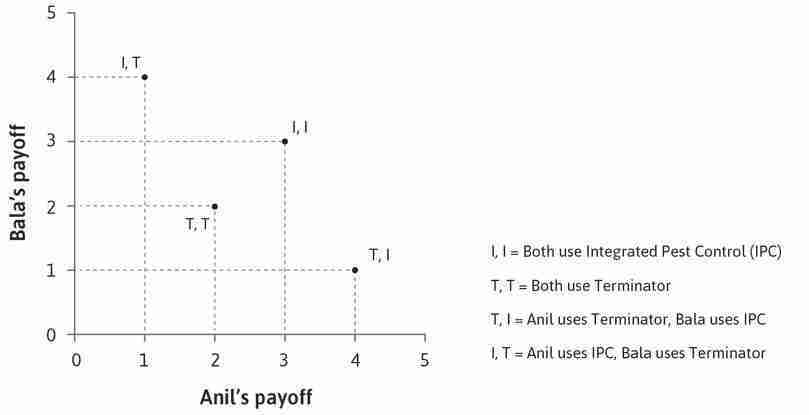
Figure 3.5 uses the Pareto criterion to compare the four allocations in the pest control game that we studied in Unit 2. In this example, we assume that Anil and Bala are self-interested, so they prefer allocations with a higher payoff for themselves. They each have two possible choices—use the chemical pesticide Terminator (T) or a non-chemical integrated pest control strategy (I). Recall that their payoffs describe a prisoners’ dilemma. Both would be better off if both used I than if both used T, but without coordination, each would be better off by choosing T, regardless of what the other does.
Pareto this and Pareto that: Make sure you understand the terms Pareto efficient, Pareto dominate and Pareto improvement. The first is a characteristic of a single allocation, the second is a comparison between two allocations, and the third is about a move from one allocation to another.
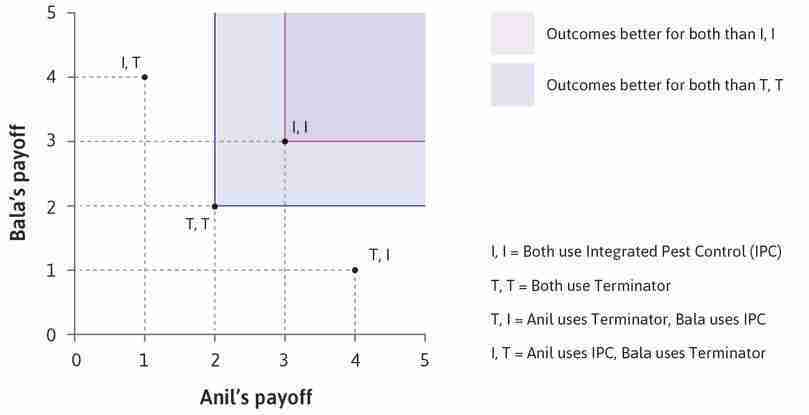
In Figure 3.5, outcome (I, I) where they each get 3 Pareto dominates (T, T) where they each get 1. Visually this is true because point (I, I) lies above and to the right of (T, T). Follow the steps in Figure 3.5 to see more comparisons.
Likewise, we can see that moving from point (T, T) to point (I, I) is a Pareto improvement, meaning that the second point Pareto dominates the first.
Pareto-efficient allocations: All of the allocations, except mutual use of the pesticide (T, T), are Pareto efficient.
Figure 3.5 Pareto-efficient allocations: All of the allocations, except mutual use of the pesticide (T, T), are Pareto efficient.
Anil and Bala’s prisoners’ dilemma
The diagram shows the payoffs in the four possible allocations when Anil and Bala play the pest control game, a prisoners’ dilemma.
Figure 3.5a The diagram shows the payoffs in the four possible allocations when Anil and Bala play the pest control game, a prisoners’ dilemma.
A Pareto comparison
(I, I) lies in the rectangle to the northeast of (T, T), so an outcome where both Anil and Bala use IPC Pareto dominates one where both use Terminator, so (I, I) is Pareto efficient.
Figure 3.5b (I, I) lies in the rectangle to the northeast of (T, T), so an outcome where both Anil and Bala use IPC Pareto dominates one where both use Terminator, so (I, I) is Pareto efficient.
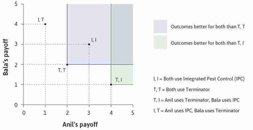
Compare (T, T) and (T, I)
If Anil uses Terminator and Bala IPC, then he is better off but Bala is worse off than when both use Terminator. The Pareto criterion cannot rank these two outcomes—neither allocation Pareto-dominates the other.
Figure 3.5c If Anil uses Terminator and Bala IPC, then he is better off but Bala is worse off than when both use Terminator. The Pareto criterion cannot rank these two outcomes—neither allocation Pareto-dominates the other.
You can see from this example that the Pareto criterion may be of limited help in comparing allocations. Here, it tells the policymaker or citizen only to rank (I, I) above (T, T).
3.5 Adding the option of transferring payoffs between players
The Pareto criterion is unhelpful to policymakers because:
- Few Pareto improvements: For major choices that policymakers and citizens face, there are very few changes that are truly win-win. And so, because there are losers from almost any policy change, a change in the status quo is almost never a Pareto improvement.
- Compensation: The Pareto criterion as we have applied it so far does not take account of the possibility that a game could have a second stage. In this stage, some of the payoffs of one player could be transferred to the other. This would more than compensate the other player for the loss in the first stage, leaving both of them better off than in the status quo.
To see how this could work, suppose the only two possible outcomes in the pest control game were option A, in which both used Terminator (T, T), or option B in which Anil used Terminator and Bala used IPC (T, I). The Pareto criterion does not rank the two outcomes: at (T, T), the two have identical payoffs, while at (T, I), Anil does much better and Bala worse. So if (T, T) were the status quo, then moving to (T, I) would not be a Pareto improvement.
But a policymaker might set aside the Pareto criterion and just look at the total of the two payoffs, namely 4 at (T, T) and 5 at (T, I). If the policymaker could choose which outcome to implement, she might choose (T, I) with the proviso that Anil will pay Bala 1.5. Then both would receive 2.5, which is better for each than at (T, T). The transfer from Anil to Bala could take the form of a tax on Anil’s income that would be transferred to Bala. Call this policy ‘(T, I) plus tax and transfer’. The result of this policy when implemented Pareto dominates the outcome (T, T). So the (T, I) plus tax and transfer outcome is Pareto efficient.
Variants of the tax and transfer policy would also Pareto dominate (T, T) as long as the amount transferred to Bala was at least 1 (so he would be better off than at (T, T)) and not greater than 2 (so that Anil would be better off than at (T, T)).
Applying a similar tax and transfer policy to the (I, T) outcome—with Bala paying Anil—would Pareto dominate (T, T).
Public policies often combine a change in the allocation (stage one of the game) followed by a transfer to compensate those whose payoffs were reduced in the new allocation (stage two).
For example, the reduction of import tariffs as part of international trade liberalization aims to create winners by making imported goods less expensive. The losers are those working in the industries that make goods that compete with similar imported goods. A policymaker might decide to compensate the losers by providing retraining and relocation opportunities for workers affected by factory closures, and some countries do this. But, in practice, trade liberalization polices have rarely been bundled with compensation policies that leave the losers no worse off as a result.
Great economists Vilfredo Pareto
He is mostly remembered for the concept of efficiency that bears his name. Suppose that we want to compare two possible allocations, A and B, that may result from an economic interaction. Can we say which is better? Suppose we find that everyone involved in the interaction would prefer Allocation A. Then most people would agree that A is a better allocation than B. This criterion for judging between A and B is called the Pareto criterion. According to the Pareto criterion, Allocation A dominates Allocation B if at least one party would be better off with A than B and nobody would be worse off. Allocation A is called Pareto efficient if there is no other allocation that is feasible—given the available resources, knowledge, and technologies—and that dominates A.
Pareto wanted economics and sociology to be fact-based sciences, similar to the physical sciences that he had studied when he was younger.
His empirical investigations led him to question the idea that the distribution of wealth resembles the familiar bell curve, with a few rich and a few poor in the tails of the distribution, and a large middle-income class. In its place he proposed what came to be called Pareto’s law, according to which, across the ages and differing types of economy, there were very few rich people and a lot of poor people.
His 80–20 rule—derived from Pareto’s law—asserted that the richest 20% of a population typically held 80% of the wealth. Were he living in the US in 2018 he would have to revise that to 90% of the wealth held by the richest 20%, suggesting that his law might not be as universal as he had thought.
Question 3.3 Choose the correct answer(s)
Which of the following statements about the outcome of an economic interaction is correct?
- Pareto efficiency has nothing to do with fairness, and it is possible for a Pareto-efficient outcome to be more unfair than a Pareto-inefficient one. For example, in the pest control game, (T, I) is efficient but less fair than (T, T).
- Pareto-efficient allocations can be very unfair, in which case it is likely that at least one participant would not be happy with the outcome.
- If the allocation is Pareto efficient, there is no allocation that Pareto dominates it; that is, no allocation where someone is better off without others being worse off.
- There can be more than one Pareto-efficient outcome. We saw that three of the four allocations in the pest control game were Pareto efficient.
Question 3.4 Choose the correct answer(s)
Peter, John, and James are discussing how to share three apples and three oranges. Which of the following statements regarding Pareto-efficient allocations is correct?
- If all of them like apples and oranges, there are at least three Pareto-efficient allocations—Peter, John, or James has all the fruits. There are also other more equitable Pareto-efficient allocations.
- Pareto efficiency is when you cannot make anyone better off without making someone else worse off. This is true when one person has all the wealth.
- This depends on their preferences. It may be that Peter loves apples but hates oranges, while John’s preference is the opposite. Then they can both be better off if Peter trades his orange for John’s apple.
- Given any allocation, it is not possible to make someone better off (giving them another fruit) without making someone else worse off (taking that fruit away).
3.6 Evaluating an outcome: Is it fair?
When combined with compensating those losing out from a policy change, the Pareto criterion can be used for a much wider set of policy problems.
Being fair does not mean automatically compensating losers. Imagine that it becomes possible for a hospital in Europe, funded by general taxation, to have its X-rays examined by qualified radiologists in Asia. This is cheaper for the hospital, which is short of funding. One group of losers would be well-paid radiologists in the hospital who lose a small part of their income as a result, and who ask that the government compensates them. It would be possible for the policymaker to replace this lost income to the hospital radiologists, and for the hospital to still save a small amount of money, although much less than before.
But policymakers faced with winners and losers may knowingly advocate a policy change that is not a Pareto improvement. Instead, they may advocate a policy on the grounds of fairness. This would be the case, for example, if those who gained were less well off and greatly in need of additional income, whilst those who lost, like the well-paid radiologists in the example, were wealthy. So far, our evaluation of outcomes has missed out fairness.
Too much inequality?
One of the reasons inequality is seen as a problem is that many people think there is too much of it.
Michael Norton, a professor of business administration, and Dan Ariely, a psychologist and behavioural economist, asked a large sample of Americans how they thought the wealth of the US should be distributed. What fraction of US wealth, for example, should go to the wealthiest 20%? They also asked them to estimate what they thought the distribution of wealth actually was.
Figure 3.6 gives the results, with the top three bars showing the distribution that different groups of responders considered would be ideal, and the fourth bar showing the wealth distribution that they thought actually existed in the US.
The top bar shows that Americans thought that, ideally, the richest 20% should own a little more than 30% of total wealth—some inequality was desirable, but not a lot. Contrast this with the fourth bar (labelled ‘Estimated’), which shows that they thought that the richest 20% owned about 60% of the wealth.
The bottom bar shows the actual distribution. In reality, the richest fifth owns 85% of the wealth. The actual distribution is much more unequal than the public’s estimate—and contrasts sharply with the lower inequality they would like to see.
Different groups largely agree on the ideal distribution of wealth. Americans with an annual income greater than $100,000 thought that the share going to the top 20% should be slightly larger than those who earned less than $50,000 thought it should be. Democratic Party voters wished for a more equal distribution than Republican Party voters, and women preferred more equality than did men, although we have not shown this information in Figure 3.6 because the differences between these groups were small. Americans, whether rich or poor, Republican or Democrat, think that the distribution of wealth should be a lot more equal than it is.
Americans’ ideal, estimated, and actual distribution of wealth.
Figure 3.6 Americans’ ideal, estimated, and actual distribution of wealth.
Adapted from Figures 2 and 3 in Michael I. Norton and Dan Ariely. 2011. ‘Building a Better America—One Wealth Quintile at a Time’. Perspectives on Psychological Science 6 (1): pp. 9–12.
Fair inequality or a tilted playing field?
Not all economic inequalities are unfair. Think of the difference in income between two identical twin brothers. The first is a poet who works part-time as a primary school teacher for a low wage, while preserving enough free time for his passion (poetry). The second is an engineer who puts in 60-hour weeks at a job that he does not enjoy so he can take home a high salary that supports his love of surfing holidays in exotic locations.
Both had opportunities for a good education. The poet dropped out after two years in university, while the surfer earned a postgraduate degree. The engineer-surfer earns three times what the poet lives on, but few people would think that the difference in income is unfair. This example shows there are more sources of inequality than the economic advantages resulting from the accidents of birth that people tend to think of as unfair.
The comparison of the brothers highlights the role of the choices made by two individuals who started at the same point on a level playing field. By making different choices, they end up with different incomes. Luck could also play a role. People will differ in their judgement about whether inequality arising from chance is fair or not.
Suppose we accept the idea that the kind of inequality that occurs between identical twins is not unfair. After all, they have the same parents and thus they win a similar prize in the lottery of accidents of birth. In our example, they grow up in the same neighbourhood, experience the same upbringing, share an identical genetic inheritance from their parents, and go to the same school.
The same reasoning applies to economic differences among identical twin sisters—but not between brother and sister twins because brother–sister differences in income could be the result of gender discrimination.
- tax
- A compulsory payment to the government levied, for example, on workers’ incomes (income taxes) and firms’ profits (profit taxes) or included in the price paid for goods and services (value added or sales taxes).
Christina Fong, an economist, wanted to know if people in the US think this way when it comes to their political support or opposition to policies to raise the incomes of the poor, financed by general taxation. An unusual survey from 1998 provided the data she needed; respondents were asked the usual questions about their economic situation, but also their opinion on why some people get ahead in life and succeed while others do not, and whether the government should introduce ‘heavy taxes’ to redistribute income to the poor.
She found that a person who thinks that hard work and risk-taking are essential to economic success is much less likely to support redistribution to the poor than a person who thinks that the key to success is inheritance, being white, your connections, or who your parents are.
The results of her study are in Figure 3.7. Notice that white people who think that being white is important to getting ahead strongly support redistribution to the poor—evidently because they think that the process that determines economic success is unfair.
How Americans’ beliefs about what it takes to get ahead predict their support or opposition to government programs to redistribute income to the poor.
Figure 3.7 How Americans’ beliefs about what it takes to get ahead predict their support or opposition to government programs to redistribute income to the poor.
Figure 5.3 in Samuel Bowles. 2012. The New Economics of Inequality and Redistribution. Cambridge: Cambridge University Press; Christina Fong, Samuel Bowles, and Herbert Gintis. 2005. ‘Strong Reciprocity and the Welfare State’. In Handbook of Giving, Reciprocity and Altruism. Serge-Christophe Kolm and Jean Mercier Ythier (eds). Amsterdam: Elsevier.
Exercise 3.3 Using Excel: Your ideal income distribution
Download and save the spreadsheet containing the data for Figure 3.6.
Using the columns provided, fill in the row labelled ‘Your own’ according to your ideal income distribution for your own country. (For example, if you think the top 20% in your country should have 40% of the income, type 40.0 into cell B7).
Plot your ideal income distribution alongside the other income distributions as a stacked bar chart in Excel. Follow the walk-through below on how to do stacked bar charts in Excel. Is your ideal income distribution similar to or different from the Americans’ ideal distribution (top three bars in Figure 3.6)?

Making a stacked bar chart.
Figure 3.8 Making a stacked bar chart.
The data
We will be using this data to create a stacked bar chart. Each row contains a particular income distribution, and each column contains a particular group of society. The last row (cells shaded blue) contains an example of how you could fill in your ideal income distribution.
Figure 3.8a We will be using this data to create a stacked bar chart. Each row contains a particular income distribution, and each column contains a particular group of society. The last row (cells shaded blue) contains an example of how you could fill in your ideal income distribution.

Draw a stacked bar chart
The stacked bar chart will look like the one shown above. If you selected the labels in Row 1, your legend would be labelled correctly. Otherwise, you have to change the labels manually.
Figure 3.8b The stacked bar chart will look like the one shown above. If you selected the labels in Row 1, your legend would be labelled correctly. Otherwise, you have to change the labels manually.
Change the legend and horizontal axis labels
The bars corresponding to the quintiles are currently named ‘Series 1’, ‘Series 2’ and so on. We need to edit their names to correspond to those in Figure 3.6.
Figure 3.8c The bars corresponding to the quintiles are currently named ‘Series 1’, ‘Series 2’ and so on. We need to edit their names to correspond to those in Figure 3.6.
Question 3.5 Choose the correct answer(s)
Figures 3.6 and 3.7 indicate that:
- The opposite is true: Figure 3.6 shows that the estimated income distribution is more equal than the actual income distribution in the US.
- The second and third bars of Figure 3.6 show that there is a noticeable difference in the ideal income of the bottom 20% (Americans whose income is < $50,000 think the bottom 20% should ideally have a larger share of income).
- Figure 3.6 shows that people think there is too much inequality in society. Figure 3.7 shows that people who believe that economic success is largely determined by ‘unfair’ processes are more likely to support redistribution policies.
- Figure 3.7 shows that support for redistribution is greater when people believe that risk-taking, rather than hard work, determines success.
3.7 Why are (some) economic inequalities unfair? Procedural and substantive judgements
Inequalities among people go beyond economic differences, and concerns about fairness are not the only basis of objections to inequality.
When people express the view that there is too much inequality, they usually refer to differences among people in one or more of the following dimensions:
- Income: The reward in money (or some equivalent measure) of the individual’s command over valued goods and services.
- Hourly pay: The income reward for a given amount of work.
- Health status: For example, longevity.
- Happiness: Economists, psychologists, and others have developed indicators by which subjective wellbeing can be measured.
- Freedom: The extent that one can do (or be) what one chooses without narrow socially imposed limits.
- Respect, dignity or social status.
Many people also object to economic inequalities—especially extreme disparities—whatever the source, on grounds other than fairness, including:
- People should have second chances: Mistakes made early in life—not working hard in school, for example—should not consign an individual to a lifetime of low income.
- Economic inequalities may undermine democracy.
- Dignity and respect matter in society: Large economic differences among people make it more difficult to achieve this.3
But we will focus here on why some economic inequalities, notably of income and wealth, are considered to be unfair.
Evaluating fairness using the veil of ignorance
The American philosopher John Rawls (1921–2002) devised a way to clarify our own ideas of fairness that can sometimes help us to find common ground on questions of values. Consider the following situation. You and a friend are walking down an empty street and you see a $100 note on the ground. How would you split your lucky find? We follow three steps:
- Fairness applies equally to all people taking part in the interaction: Whatever the rule for dividing up the $100 is, it cannot involve the identity of one or the other of the players. (This principle, for example, would reject as unfair the rules of the game of a monarchy, in which a named person, say George III, is head of state; democratic constitutions specify how the head of state is to be selected, not who this will be.)
- Imagine a veil of ignorance: Since fairness applies to everyone, including ourselves, Rawls asks us to imagine ourselves behind what he called a veil of ignorance, not knowing the position that we would occupy in the society we are considering. We could be male or female, healthy or ill, rich or poor (or with rich or poor parents), in a dominant or an ethnic minority group, and so on. In the $100 on the street game, we would not know if we would be the person picking up the money, or the person responding to the offer.
- From behind the veil of ignorance, we can make a judgement: For example, the choice of a set of institutions—rules of the game that will determine who gets what—imagining that we will then become part of the society we have endorsed, with an equal chance of having any of the positions occupied by individuals in that society.
In making a judgement about fairness, the veil of ignorance assists you in doing something very difficult: putting yourself in the shoes of others quite different from you. You would then, Rawls argued, be better able to evaluate the constitutions, laws, inheritance practices, and other institutions of a society as an impartial outsider.
The veil of ignorance is a way of looking at problems of inequality and justice, it is not a statement about what is fair and what is not.
- substantive judgements of fairness
- Judgements based on the characteristics of the allocation itself, not how it was determined. See also: procedural judgements of fairness.
- procedural judgements of fairness
- An evaluation of an outcome based on how the allocation came about, and not on the characteristics of the outcome itself, (for example, how unequal it is). See also: substantive judgements of fairness.
The two studies of Americans’ attitudes towards fairness that we looked at in the previous section make a basic point about how people judge differences in these dimensions. Allocations can be judged unfair because of:
- How unequal they are: In terms of income, for example, or subjective wellbeing or the distribution of wealth, in Figure 3.6. These are substantive judgements of fairness.
- How the inequalities came about: For example, by force or racial discrimination, by competition on a level playing field, or by hard work, as in Figure 3.7. These are procedural judgements of fairness.
Substantive judgements
These are evaluations of the allocation itself—the shares of the pie. We know from the behaviour of ultimatum game experimental subjects (Figure 3.2) that many people would judge as unfair an allocation in which the Proposer took 90% of the pie. That is a substantive judgement about unfairness of an economic inequality.
To make a substantive judgement about fairness, all you need to know is the allocation itself; you do not need to know the rules of the game and other factors that explain why this allocation occurred.
Suppose you lived in a society in which one segment of the population had limited access to medical care and as a result they had high rates of illness, high child mortality and limited life expectancy. Others in the same population had excellent medical care including access to cosmetic surgery and other vanity medical treatments. You might decide this situation was unfair.
But what is unfair about it?
One answer is that by reallocating medical personnel and facilities a vast improvement in the medical care of the disadvantaged group could be accomplished without any significant reduction of the health of the advantaged group. By this reasoning an unequal economic outcome is unfair if reducing the inequality would substantially increase the wellbeing of the poorer group, without inflicting significant reductions in wellbeing of the better-off group.
This view is based on a comparison of the wellbeing (or ‘utility’) of individuals and how it is affected by a change in the resources available to them. Its origins are with the utilitarian economist and philosopher, Jeremy Bentham (1748–1832). We could call this ‘utilitarian unfairness’ or Bentham-unfairness.
A second (and quite different) view of the unfairness of the inequality was put forward by John Rawls in an essay titled Justice as Fairness. Rawls held that in addition to equal rights and liberties, and equality of opportunity to better yourself, a just society is one in which the least well-off group are as well off as they can be.4 Where this is not true, we have what we will call ‘Rawls-unfairness’.
This does not imply that economic inequalities can never be just, or that equality of income or wealth is the standard against which to judge unfairness. If paying doctors more than others is necessary to provide them with incentives to address the health needs of the poorest, then their higher incomes does not violate Rawls-unfairness.
Procedural judgements
These are ideas of fairness based on how the inequality came to be that focus not on how poor or rich someone is, but instead on why the person is poor or rich.
The rules of the game that brought about the inequality may be evaluated according to aspects such as:
- Voluntary exchange of private property acquired by legitimate means: Were the actions resulting in the allocation the result of free choices by the individuals involved? For example, did each person buy or sell things that they had come to own through inheritance, purchase, or their own labour? Or was fraud or force involved?
- Equal opportunity for economic advantage: Did people have an equal opportunity to acquire a large share of the total, or were they subjected to some kind of discrimination because of their race, sexual preference, gender, or who their parents were?
- Deservingness: Did the rules of the game that determined the inequality take account of the extent to which individuals need, or for some other reason deserve, the amounts they get?
We can use these differing judgements to evaluate an outcome in the ultimatum game. The experimental rules of the game will appear to most people’s minds as procedurally fair:
- Proposers—who can expect to receive not less than half of the pie, and will probably receive more—are chosen randomly.
- The game is played anonymously, so who a person is (her name, or title, or some other aspect of her identity) cannot matter.
- All actions are voluntary. The Responder can refuse to accept the offer, and the Proposer is typically free to propose any amount.
These rules of the game are (procedurally) fair. But, as we have seen, the actions of Proposers are often seen as (substantively) unfair.
Now imagine that the person selected to be Proposer was based on ethnic origin and gender so that only males of European origin can be the Proposer. The game would be procedurally unfair by awarding the position that has the greatest income-earning prospects using a rule that discriminates against women and non-Europeans.
This suggests that, for many people, the question, ‘How much inequality is too much?’ cannot be answered unless we know why a family or person is rich or poor. Many people think it is unfair if income depends substantially on accidents of birth, such as your race, your sex, or your country. Inequalities based on hard work or taking risks are less likely to be seen as unfair.
A video of economist Helen Miller speaking to students at Manchester University in the UK in 2017 outlines some of the issues of tax fairness, starting with the question, ‘What would be a fair tax rate for George Harrison?’. (George Harrison was lead guitarist for The Beatles during the 1960s and 1970s. The Beatles were the world’s most famous pop group at the time. He was a high earner which meant that some of his income was taxed at a rate of 95%.)
George Harrison had such a strong opinion about the unfairness of the 95% marginal tax rate that he wrote and recorded a song with the Beatles called ‘Taxman’ in 1966. It includes the lyrics, ‘Let me tell you how it will be/There’s one for you, 19 for me’.
Neither philosophy, economics, nor any other science, can eliminate disagreements about questions of value. But economics can clarify:
- How the dimensions of unfairness may be connected: For example, how the rules of the game that give special advantages to one or another group may affect the degree of inequality of income.
- Trade-offs between the objectives of fairness and efficiency: For example, are some kinds of unfairness essential for achieving efficient outcomes? Does unfairness (as in the ultimatum game) sometimes lead to inefficient outcomes (remember that the money is thrown away if the offer is rejected).
- Public policies to address concerns about unfairness: How can unfairness be reduced by the actions of governments and other bodies?
- The effects of the introduction of new policies: Economics can measure this once businesses, individuals, and other private economic actors have responded to the opportunities and constraints imposed by the new environment, and then use this information to make better policies in future.
The last bullet point poses our next challenge—will the intended outcomes of a government policy result once we take account of not only government actions, but also the reactions of private actors?
Exercise 3.4 Substantive and procedural fairness, and the veil of ignorance
Consider the society you live in, or another society with which you are familiar.
- To make society fairer (according to the substantive judgement of fairness), would you want greater equality of income, happiness, or freedom? Why? Would there be a trade-off between these aspects?
- Are there other things that should be more equal to achieve greater substantive fairness in this society?
- How fair is this society, according to the procedural judgement of fairness?
- Suppose that, behind a Rawlsian veil of ignorance, you could choose to live in a society in which one (but only one) of the three procedural standards for fairness (voluntary exchange of property, equality of opportunity, and deservingness) would be the guiding principle for how institutions are organized. Which procedural standard would you choose, and why?
Question 3.6 Choose the correct answer(s)
Which of the following statements regarding substantive judgements of fairness is correct?
- Substantive judgements may be based on the individual’s freedom, in other words, the extent that one can do (or be) what one chooses without socially imposed limits.
- Fairness may depend on the individual’s happiness rather than income. One may think that a person with a serious disability requires more income than those without to be equally satisfied with his life.
- Economists have developed indicators to measure subjective wellbeing. Although these measures are imperfect, they enable us to use happiness as a criterion to evaluate allocations.
- They may disagree if they use different criteria to evaluate the situation. For example, one may evaluate fairness in terms of income, and the other may do so in terms of happiness.
Question 3.7 Choose the correct answer(s)
Which of the following statements regarding procedural judgements of fairness is correct?
- There is inequality in the opportunity for economic advantage, namely that only those with university degrees can be the Proposer (who would typically gain more of the pie than the Responder). Therefore, the game is not procedurally fair.
- Procedural judgements of fairness may consider deservingness—do the rules of the game that determine the allocation reflect what the social norm states regarding deservingness?
- It may be that a substantively unfair outcome (for example, unequal allocation) arises through a procedurally fair process (for example, voluntary exchanges).
- For example, using threats to attain income equality may be substantively fair but not procedurally fair.
3.8 Implementing public policies
Giving women the vote reduced child deaths in the US. Requiring randomly selected Indian villages to be headed by women changed spending priorities in ways that benefited women.
Governments implement policies through some combination of:
- Prohibitions and directives: Some actions can be simply directed by the government (sending your children to school) or prohibited (using leaded fuel for your car).
- Incentives: A policy changes the benefits or costs of alternative courses of action open to the individual.
- Making information available: People can use this information when they make decisions about which actions to take.
There is a limit to the extent that governments can order people around, and this is a problem for government policymakers. Even something simple, like imposing a speed limit on a highway, does not prevent people from driving fast. It just changes the environment in which the driver’s decision about how fast to drive occurs.
For this reason, the outcome of a government policy is not something the government can dictate. Instead, it is the result of an interaction between the government’s actions and the privately chosen actions of those affected.
- Nash equilibrium
- A set of strategies, one for each player in the game, such that each player’s strategy is a best response to the strategies chosen by everyone else.
To understand how government policies can change economic outcomes by changing what actions people decide to take, we will use game theory and the idea of a Nash equilibrium, introduced in Section 2.11. Recall that a Nash equilibrium is a set of strategies adopted by players such that each is a best response to the others, so that none of the players have an incentive to change their strategy.
Nash equilibrium and Pareto efficiency are both concepts used in public policy analysis, but keep in mind that they refer to entirely different aspects of a social interaction. Figure 3.9 clarifies the relationship between the two concepts by using the invisible hand (crop selection) and pest control games.
| Pareto efficient | Not Pareto efficient | |
|---|---|---|
| Nash equilibrium | Anil grows cassava, Bala grows rice (Invisible hand game) | Both use Terminator rather than IPC (Pest control game) |
| Not a Nash equilibrium | Both use IPC; or one uses Terminator, the other IPC (Pest control game) | Bala grows cassava, Anil grows rice; or both grow the same crop (Invisible hand game) |
Pareto efficiency and Nash equilibrium contrasted, using two games.
Figure 3.9 Pareto efficiency and Nash equilibrium contrasted, using two games.
Entries in the table are examples of the combinations indicated by the column and row names. The lower left cell, for example, indicates that three of the four outcomes in the pest control game—both use IPC, Bala uses Terminator and Anil uses IPC, and Anil uses Terminator and Bala uses IPC—are Pareto efficient, but none of the three is a Nash equilibrium.
Implementing fairness and efficiency in averting the tragedy of the commons
Let’s return again to the tragedy of the commons and make things concrete (if somewhat unrealistic at this stage). The tragedy of the commons—as you saw in Unit 2 (Section 2.2)—can be represented as a prisoners’ dilemma in which overgrazing is the dominant strategy, even though restricting the amount of grazing would support higher payoffs for both players.
Let’s say there are just two herders, and that they may each put either 10 or 20 cows on the communal pasture. The payoff table for their interaction is shown in Figure 3.10.
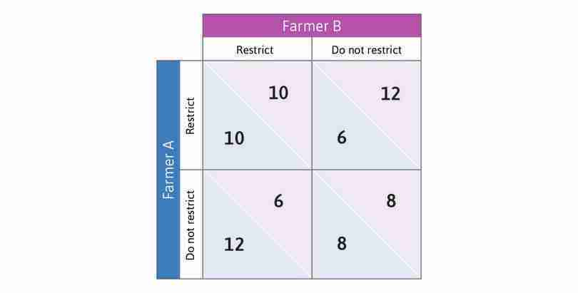
Overgrazing the commons.
Figure 3.10 Overgrazing the commons.
You can confirm that this is a prisoners’ dilemma by noticing that whatever B does—restrict the cows she places on the commons to 10 or not—the highest payoff for A is to place 20 cows on the pasture. By pasturing more cows, she gets 12 rather than 10 if B has restricted his cows to 10, or 8 rather than 6 if he has pastured 20 cows.
The same is true of B. Whatever A does, the best for him is to put 20 cows on the pasture. Yet both A and B would be better off—getting 10 rather than 8—by both restricting the number of cows they put to pasture. Overgrazing is the Nash equilibrium.
An effective government policy might alter this situation by changing the Nash equilibrium. But how can this be done?
A tax on overgrazing to change the Nash equilibrium
We saw at the beginning of this unit that one solution would be to give A access to the pasture and exclude B. This alters the game fundamentally. She would then pasture all 20 of her cows there, B would pasture none, and A would get a payoff of 20 (and B would get zero). While this solved the problem of overgrazing, it seemed unfair to B.
But the government could pursue a more even-handed approach. The problem of overgrazing, remember, arises because each herder, when deciding on how many cows to keep, thinks only of his or her own payoffs. Thus, when A compares pasturing 20 cows as opposed to 10 where B is pasturing only 10, she looks at how her own payoff is affected, rising from 10 to 12 as she adds the extra cows. She does not look at the fact that B has just seen his payoffs drop from 10 to 6. A has ignored the costs that her action imposed on B.
If A were altruistic, she might be concerned about the harm she caused B, and not overgraze. If the two were close friends or relatives, this might be enough to prevent overgrazing. Instead, let’s imagine they are complete strangers and do not care at all for each other. As we saw in Unit 2 in the game with Anil and Bala, if there were really only two people involved, they probably would not be complete strangers, but we are using the two-person case as a simplification to understand what happens when there are dozens or even hundreds of herders, among whom many would be unknown to each other.
The government, however, could address the problem by adopting a policy that imposed a tax of 0.4 for any cow beyond 10 that a herder sent to pasture. We assume that the government uses the tax revenues for some purpose unrelated to the problem of overgrazing. This just means we do not have to think about what the tax is spent on. Under this new tax policy, for example, either herder would pay a tax of 4 if the herder sent 20 rather than 10 cows to pasture. The ‘overgrazing tax’ changes the payoff matrix, as shown in Figure 3.11.
An overgrazing tax averts the tragedy of the commons.
Figure 3.11 An overgrazing tax averts the tragedy of the commons.
The original situation
In Figure 3.10 (reproduced here), overgrazing occurred because each herder ignored the cost of their actions on the other herder. The Nash equilibrium is (Do not restrict, Do not restrict).
Figure 3.11a In Figure 3.10 (reproduced here), overgrazing occurred because each herder ignored the cost of their actions on the other herder. The Nash equilibrium is (Do not restrict, Do not restrict).
An overgrazing tax
Imposing the overgrazing tax reduces the payoffs for ‘Do not restrict’ by 4, making (Restrict, Restrict) the Nash equilibrium. The commons is protected.
Figure 3.11b Imposing the overgrazing tax reduces the payoffs for ‘Do not restrict’ by 4, making (Restrict, Restrict) the Nash equilibrium. The commons is protected.
The effect of the tax is to displace the Nash equilibrium from each herder putting 20 cows on the commons to both of them putting only 10. You can check that protecting the commons is now a Nash equilibrium—when one is putting only 10 cows on the commons the best response of the other is to also put only 10 cows on the commons.
The overgrazing tax has three valued features:
- It treats both herders equally: It averts the tragedy without introducing inequality among the herders and so, in this sense, it is both efficient and fair.
- Each herder must take account of the cost that their overgrazing imposes on the other: Note they do not have to care about the other herder because the cost is a tax on each herder.
We assumed both herders are the same. There is an additional feature of the tax that would occur if some are better at cattle raising than others.
- The better herders will find it more valuable to put their cows on the pasture: Those less skilled at raising cattle will not find it worth paying the tax. As a result, the better herders will have greater access to the pasture.
This solution is efficient—those who can make the best use of the land are using it. Any decision about whether this is fair or not would depend on additional facts that we have not discussed, for example, whether the not-so-good herders are better at something else, and whether they can make their living without herding.
But often it is more difficult to fashion a policy that will achieve its objectives, as the examples in the next two sections show.
Question 3.8 Choose the correct answer(s)
Which of the following statements about the tragedy of the commons shown in Figure 3.11 is correct?
- The herders are still self-interested, but the overgrazing tax changes their incentives to account for the costs they impose on each other, and hence changes the outcome.
- The overgrazing tax may not be fair if some herders are better at raising cattle than others.
- When one herder chooses to overgraze, it raises her payoff by 2 but reduces the other herder’s payoff by 4. With the tax of 4, she will now completely account for this cost imposed on the other herder.
- The overgrazing tax only changes the incentives of the herders, not the information available.
3.9 Unintended consequences of a redistributive tax
Suppose that a newly elected government wants to raise taxes on the profits of firms in order to fund high-quality public education and other new programs that will benefit middle- and low-income voters. At the current moderate tax rate, firms are making high after-tax profits. The new finance minister introduces a higher tax rate, calculating that it will raise revenue by 50%. Then he sets about planning how to spend the additional tax revenues, announcing popular improvements in pre-primary schooling.
The finance minister is not surprised when firm owners protest against the new tax rate. But he is dismayed when the head of the tax collection agency reports that tax revenues are falling. She estimates that the revenue from the profits tax will be 10% lower than it was the previous year. What has gone wrong?
The head of tax collection explains that when the tax rate went up, firms began hiring tax lawyers to exploit loopholes in the tax laws. The finance minister has failed to consider that a change in the tax regime may cause firms to change their strategies too.
The firms’ response to government policy—hire lawyers to exploit tax loopholes—is commonly adopted in real life. Recall that George Harrison objected to the taxman saying, in his words, ‘One for you, 19 for me,’ in the 1960s. The Beatles hired an accountant who explained that if they formed a company, they would not have to pay the 95% marginal income tax, because company income was taxed at a lower rate than personal income. This is what they did.
Why firms hire tax lawyers
To understand the misjudgement made by our finance minister, we can represent the interaction between government policy and the strategies of firms as a game, which we will call the tax avoidance game, played by two hypothetical people—the ‘Government’ who will levy taxes and direct their uses, and the ‘Firm owner’ who will pay taxes on the profits accruing to the firm.
The Government would like taxes (and therefore its ability to improve schools) to be greater, and the Firm would like profits after the payment of taxes (‘after-tax profits’) to be greater. Those who will benefit from the expenditure of the tax revenue—on improved pre-primary centres, for example—are not players in the game as their role is entirely passive. Their actions do not affect the payoffs of the two players.
We will assume that each of the players has just two choices. In the games we studied before, the two players had the same two strategies to choose from—plant cassava or plant rice; use integrated pest management or use the Terminator pesticide; use C++ or use Java. Here, we recognize that the actors differ—the actions open to the Government are not the same as the actions open to a private citizen or the owner of the Firm:
- The Government: May levy either moderate taxes or high taxes on the Firm owner’s profits.
- The Firm: Can either pay taxes at the statutory (government-intended) rate, or hire tax lawyers to exploit loopholes in the tax laws—finding accounting methods that will allow the Firm to ‘earn’ its profits in some other lower tax country, for example—so as to minimize its tax obligations.
The strategies available and the payoffs associated with each strategy are given in Figure 3.12. Consider first what happens when the owner pays tax at the statutory rate:
- When the tax rate is moderate: $100 million in tax is collected and the Firm’s profits are $500 million (the upper left cell, A).
- At the higher tax rate: $150 million in tax is collected (lower left cell, B) and profits fall to $450 million. This is what the finance minister had expected to happen.
Now suppose that hiring legal advisors to find tax loopholes costs $20 million; the lawyers will be able to save the firm $15 million when the tax rate is moderate, and $60 million at the high tax rate. We can calculate the payoffs in cases C and D, as shown in Figure 3.12.
Figure 3.13 shows a useful way of representing the payoffs in this game. The Government’s payoff (tax revenue) is shown on the horizontal axis, and the Firm’s payoff (profits after taxes and lawyers’ fees) on the vertical axis. Each of the four cases A, B, C and D in Figure 3.12 is marked as a point in this diagram.
Figure 3.13 tells the story of the newly elected government’s redistributive tax policy. Initially, having ‘inherited’ the tax policies of the previous government, it finds itself at point A. Work through the steps in Figure 3.13 to see what happens next.
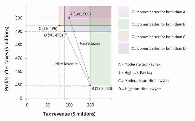
Payoffs in the tax avoidance game: How higher taxes may lead to less redistribution.
Figure 3.13 Payoffs in the tax avoidance game: How higher taxes may lead to less redistribution.
The payoffs in the four possible cases
The Government’s payoff is shown on the horizontal axis, and the Firm’s payoff on the vertical axis. The four points show the payoffs in each of the possible outcomes of the game.
Figure 3.13a The Government’s payoff is shown on the horizontal axis, and the Firm’s payoff on the vertical axis. The four points show the payoffs in each of the possible outcomes of the game.
When the Government comes into office, the tax rate is moderate
Initially the tax rate is moderate and the Firm pays the tax intended. The payoffs are shown by point A—100 for the Government and 500 for the Firm.
Figure 3.13b Initially the tax rate is moderate and the Firm pays the tax intended. The payoffs are shown by point A—100 for the Government and 500 for the Firm.
With a moderate tax rate, the Firm does not want to hire lawyers
Point C shows the payoffs if the Firm hires lawyers when the tax rate is moderate. Profits are lower at C than at A, so the Firm prefers to pay tax at the statutory rate.
Figure 3.13c Point C shows the payoffs if the Firm hires lawyers when the tax rate is moderate. Profits are lower at C than at A, so the Firm prefers to pay tax at the statutory rate.
Comparing payoffs
The pink-shaded area shows points where both players are better off than at point C. Point A lies inside this area—both the Government and the Firm are better off at A than C.
Figure 3.13d The pink-shaded area shows points where both players are better off than at point C. Point A lies inside this area—both the Government and the Firm are better off at A than C.
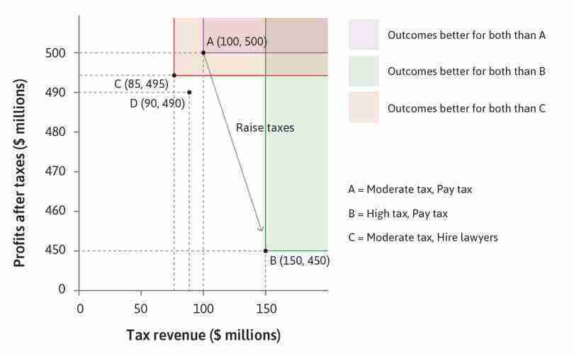
The Government raises the tax rate
The Government sets a high tax rate, hoping to move from A to B. At B, the Government is better off, but the Firm is worse off.
Figure 3.13e The Government sets a high tax rate, hoping to move from A to B. At B, the Government is better off, but the Firm is worse off.
With a high tax rate, the Firm prefers to hire lawyers
Now that the tax has risen, the Firm re-evaluates the benefits of legal advice. Hiring lawyers would change the payoffs from B to D, where profits are higher. The Firm decides to hire lawyers.
Figure 3.13f Now that the tax has risen, the Firm re-evaluates the benefits of legal advice. Hiring lawyers would change the payoffs from B to D, where profits are higher. The Firm decides to hire lawyers.
In the end, both players are worse off
The decisions of the Government and the Firm have changed the payoffs from point A to point D. Both players have lower payoffs than they had at the beginning.
Figure 3.13g The decisions of the Government and the Firm have changed the payoffs from point A to point D. Both players have lower payoffs than they had at the beginning.
Can the game help us understand the challenge facing the Government? Notice first that, at the initial moderate tax rate, the Firm is not tempted to hire lawyers. It is better off at point A, paying tax at the statutory rate, than it would be at point C. But the strategies at point A are not a Nash equilibrium; given that the Firm is not hiring lawyers, the Government does better by raising taxes, taking it to point B.
But—and this is the key point—the strategies leading to outcome B, which the Government wishes to implement, are not a Nash equilibrium either! Given the higher tax rate, the Firm does better hiring tax lawyers. And so the outcome spirals downwards from point A to B to D—where they finally reach a Nash equilibrium. At this point, both players are doing the best they can, given the strategy chosen by the other player.
Point D is dominated by point A. Sadly, both players are worse off at the Nash equilibrium D than they would have been if they had remained at A, with moderate taxes and no lawyers. Because of their decisions, after-tax profits are lower and tax revenues are lower too.
A successful policy must be a Nash equilibrium
When government officials raise tax rates, the policy often succeeds. But our analysis illustrates that the outcomes of policies are determined by the decisions of private actors as well as those government officials. The outcome that the government wants must be a Nash equilibrium. Otherwise, like point B in Figure 3.13, it will not last.
This means that once the policy is implemented—say, a new tax—the intended outcome must be the result of everyone doing the best they can, given what everyone else is doing under the new tax. If that is not the case, then people will change what they are doing, and the intended outcome of the policy will not occur.
Question 3.9 Choose the correct answer(s)
Which of the following statements about the tax avoidance game in Figure 3.13 is correct?
- It is true that outcome D is a Nash equilibrium. However, outcome A is better for both the firm and the government compared to outcome D, so outcome D is not Pareto efficient.
- There are two Pareto-efficient outcomes (A and B).
- For example, if the cost of hiring a lawyer exceeded the savings ($40 million), then firms would choose not to hire lawyers, resulting in B being a Nash equilibrium.
- If the firms saved less in taxes than they would spend in hiring a lawyer, then firms would choose not to hire lawyers, resulting in B being a Nash equilibrium.
3.10 Unintended consequences: Policies affect preferences
The tools we are developing are useful in many settings, not just so that governments can design policies. Consider the policy of an organization—a daycare centre—rather than a government.
Sometimes it is possible to conduct experiments ‘in the field’; that is, to deliberately change the economic conditions under which people make decisions, and observe how their behaviour changes. An experiment conducted in Israel in 1998 demonstrated that behaviour may be very sensitive to the context in which decisions are made.
It is common for parents to rush to pick up their children from daycare. Sometimes, a few parents are late, making teachers stay extra time. What would you do to deter parents from being late?
Two economists ran an experiment that introduced fines in some daycare centres but not in others (these were used as controls). The ‘price of lateness’ went from zero to ten Israeli shekels (about $3 at the time). Surprisingly, after the fine was introduced, the frequency of late pickups doubled. The top line in Figure 3.14 illustrates this.
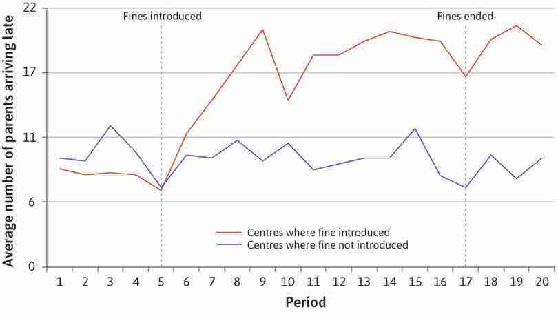
Average number of late-coming parents, per week.
Figure 3.14 Average number of late-coming parents, per week.
Uri Gneezy and Aldo Rustichini. 2000. ‘A Fine is a Price’. The Journal of Legal Studies 29 (January): pp. 1–17.
Why did putting a price on lateness backfire?
One possible explanation is that before the fine was introduced, most parents were on time because they felt that it was the right thing to do. In other words, they came on time because of a moral obligation to avoid inconveniencing the daycare staff. Perhaps they felt an altruistic concern for the staff, or regarded a timely pick-up as a reciprocal responsibility in the joint care of the child. But the imposition of the fine signalled that the situation was really more like shopping. Lateness had a price and therefore could be purchased, like vegetables or ice cream.5
The use of a market-based incentive—the price of lateness—had provided what psychologists call a new ‘frame’ for the decision, making it one in which self-interest rather than concern for others was acceptable. Before the imposition of the fine, picking up your child late, though sometimes unavoidable was a violation of a social norm. The parents’ social preferences told them to try to avoid this. The fine changed the frame: now coming late was something you could simply purchase, by paying the fine. The parent’s self-interested preferences now said: coming late is OK as long as I pay the fine (and the fine is not too high).
- crowding out
- There are two quite distinct uses of the term. One is the observed negative effect when economic incentives displace people’s ethical or other-regarding motivations. In studies of individual behaviour, incentives may have a crowding-out effect on social preferences. A second use of the term is to refer to the effect of an increase in government spending in reducing private spending, as would be expected for example in an economy working at full capacity utilization, or when a fiscal expansion is associated with a rise in the interest rate.
When fines and prices have these unintended effects, we say that economic incentives have crowded out social preferences. Even worse, you can also see from Figure 3.14 that, when the fine was removed, parents continued to pick up their children late. The new frame—lateness is something you can buy—seems to have persisted even after the fine was removed.
If the policymaker ignores how people will respond to its actions, this policy is unlikely to have its intended effect.
Sections 3.9 and 3.10 illustrate some essentials of the policymaker’s toolkit that will help to avoid unintended consequences. A good policymaker must make sure that:
- The policy does not change people’s preferences in unintended ways: A change in preferences might mean that behaviour changes too, which may mean the policy fails to hit its target. This is what happened in the daycare centres in Israel.
- The intended outcome is a Nash equilibrium: Under the new policy, people must be motivated to act in ways that are consistent with the objective of the policymaker.
Exercise 3.5 Using Excel: The effect of daycare centre fines
As in science experiments, we can think of the daycare centre experiment in terms of a ‘treatment’ and a ‘control’ group. Daycare centres who received fines were in the ‘treatment’ group, and those who did not were in the ‘control’ group.
Download and save the spreadsheet containing the data used to create Figure 3.14. You can see that Centres 1–6 are the ‘treatment’ group, while Centres 7–10 are the ‘control’ group.
Follow the walk-through in Figure 3.15 below to help you do this exercise.
The data
This is what the data looks like. Column A contains time periods, Columns B to G contain the number of late arrivals in centres where fines were introduced, and Columns J to M contain the number of late arrivals in centres where fines were not introduced.
Figure 3.15a This is what the data looks like. Column A contains time periods, Columns B to G contain the number of late arrivals in centres where fines were introduced, and Columns J to M contain the number of late arrivals in centres where fines were not introduced.
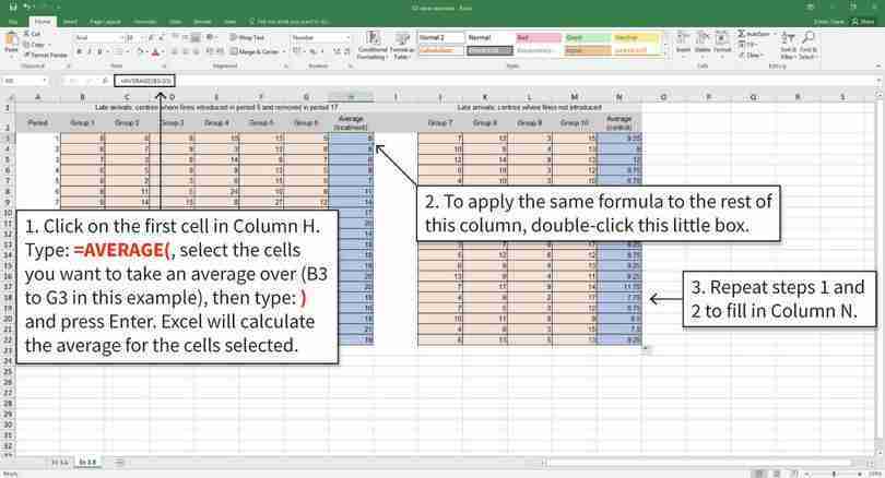
Calculate averages for each group and time period
We will use Excel’s AVERAGE function to calculate the average number of late arrivals for both groups, and put them in the shaded blue cells.
Figure 3.15b We will use Excel’s AVERAGE function to calculate the average number of late arrivals for both groups, and put them in the shaded blue cells.

Draw a line chart
After completing step 6, your line chart should look like the one shown above.
Figure 3.15c After completing step 6, your line chart should look like the one shown above.
Add dotted lines to show when fines were introduced and removed
Using Excel’s ‘Insert Shapes’ option, you can add lines to your chart. To make a line dotted, you need to change its ‘Dash type’ using the options in the right-hand menu.
Figure 3.15d Using Excel’s ‘Insert Shapes’ option, you can add lines to your chart. To make a line dotted, you need to change its ‘Dash type’ using the options in the right-hand menu.

Add text boxes to label the dotted lines
Using Excel’s ‘Insert Shapes’ option, you can add also text boxes and other shapes to your chart.
Figure 3.15e Using Excel’s ‘Insert Shapes’ option, you can add also text boxes and other shapes to your chart.

Add axis titles and a chart title
After step 15, your chart will look like Figure 3.14.
Figure 3.15f After step 15, your chart will look like Figure 3.14.
- Fill in the columns ‘Average (treatment)’ and ‘Average (control)’ by taking the average separately for each group, for each period.
- Plot a line chart of the ‘Average (treatment)’ and ‘Average (control)’. Your chart should look similar to Figure 3.14. Label the lines as in Figure 3.14.
- Calculate the difference in average lateness in Period 5 and in Period 17 (‘Average (treatment)’ minus ‘Average (control)’). Relate these numbers to what you see in your chart or in Figure 3.14.
- One explanation for the observed difference in Period 17 is that the treatment and control groups were initially different. Based on your answer to Question 3 and your Excel chart, do you think this explanation is plausible? What other aspects of the treatment and control groups do you think should be similar before the fines were introduced in order for us to infer that the fines ‘caused’ the increased lateness?
- Why do you think that, after the fine was removed, parents in the treatment group still continued to pick up their children late?
Question 3.10 Choose the correct answer(s)
Which of the following statements about the field experiment shown in Figure 3.14 are correct?
- The parents paid the fine if they were late and not otherwise; it can be considered as a price for lateness.
- The graph shows that the number of late-coming parents more than doubled in the centres where the fine was introduced.
- The crowding out of social preferences occurs when the moral obligation of not being late is replaced by the market-like incentive of purchasing the right to be late without ethical qualms. This is evident in the graph immediately after the introduction of the fines.
- The graph shows that the number of late-coming parents remained high after the fine was abolished, so it is possible that the experiment had a permanent effect.
3.11 How do we find out if a policy will work?
We have seen that a policy works by changing a Nash equilibrium. In other words, it works by changing people’s behaviour when they are doing the best they can, considering the new policy and what everyone else is doing (including the policymaker).
Thus, the policymaker faces another real-world policy design problem. When the policymaker pulls the policy lever, how do we work out the effect on outcomes? So far, we have simplified by assuming that our policymaker knows the possible futures with certainty—how the policy will shift the Nash equilibrium, and so what the outcome will be. This meant we could fill in the payoffs in the payoff matrix.
Policymakers sometimes talk of policy ‘levers’ or ‘dials’, but the connection between the policy and the effect is rarely as simple as these mechanical terms suggest.
If the policy makes something illegal, such as banning the use of lead in petrol, we can assume it will (broadly) be obeyed. But, in most cases, we do not know with this level of precision what the impact of a policy would be. If a tax is imposed on sugary drinks to discourage obesity and prevent diabetes, how do we know if people will drink tomato juice instead, or just switch to eating more chocolate to get their sugar? We also do not know how the effect might differ among, say, the rich and poor.
This is a challenge because the effect of a policy often depends on the actions taken by millions of people. We could ask each of them, ‘If a soft drink were to cost you an additional euro per can, how would that change the amount you drink in a week?’ But we should not be confident that we would get a reliable answer.
There are ways of narrowing the range of uncertainty about the effects of policies. Rather than asking people, economists typically look at what people do. First, we can examine the effects of similar policies adopted in the past, or by other bodies. This is why policymakers in India assumed that having women in political leadership in Indian villages would affect the decisions that were made.
But it is often difficult to distinguish between the effects of the policy under consideration, and the effects of other things that happened to take place at the same time. For example, see Figure 3.16.
Before introducing a sugar tax, a government may consult medical evidence about the problem of diabetes and its links to sugar consumption, and use it to explain to the public why it is considering the tax. Now imagine that sugary drink consumption falls following the tax. This might have happened because the drinks are more expensive. But it might also be because the public has new information about the effect of sugar, and this had the effect, not the higher price.
In this case, the correct policy would have been to provide information, not to impose the tax.
Here are two cases illustrating how researchers have estimated the effects of policies, starting with food taxes designed to reduce obesity.
The impact of taxes on food
Taxes on food will raise its price. The ability to measure how the amount sold varies in response to a change in price is essential for policymakers.
- price elasticity of demand
- The percentage change in demand that would occur in response to a 1% increase in price. We express this as a positive number. Demand is elastic if this is greater than 1, and inelastic if less than 1.
The effect of the tax will depend on what is termed the price elasticity of demand. This is the percentage change in demand (the amount sold) divided by the percentage change in price, made into a positive number (it will be negative, because demand goes down when prices go up).
- If demand is highly elastic: A small increase in price will cause a large reduction in sales, and the number is high (even greater than 1 in some cases). Typically, luxury or fun foods have elastic demand, because they are easier to do without.
- If demand is inelastic: Food which we consider essential for our diet has a low elasticity of demand, meaning that we continue to buy it in similar quantities when the price goes up. When demand is inelastic, the percentage change in demand is very low, and so elasticity is close to zero.
Note that policies applied to taxes on food (and all other goods that we buy, such as alcohol and petrol) have different effects depending on the price elasticity of demand:
- Taxes on inelastic demand mostly raise government revenues: A government wishing to raise tax revenue should choose to tax products with inelastic demand, because we will continue to buy them. For centuries, governments around the world—including France, Russia, China, and the British Empire (in India)—have taxed salt. Consumers do not cut back much on their salt consumption. Its demand is highly inelastic, so substantial revenues could be collected.
- Taxes on elastic demand mostly change consumer behaviour: A government wishing to change our food choices should choose to tax those foods and drinks with the most elastic demand. This is the reasoning behind a sugar tax.
Anti-obesity taxes in practice
Several countries, including Mexico and France, have introduced taxes intended to reduce the consumption of unhealthy food and drink. A 2014 international study found worrying increases in adult and childhood obesity since 1980. In 2013, 37% of men and 38% of women worldwide were overweight or obese. In North America, the figures were 70% and 61% respectively, but the obesity epidemic does not only affect the richest countries—the corresponding rates were 59% of men and 66% of women in the Middle East and North Africa.
Matthew Harding and Michael Lovenheim used detailed data on the food purchases of US consumers to estimate elasticities of demand for different types of food, to investigate the effects of food taxes. They divided food products into 33 categories and used assumptions about how consumers make decisions to examine how changes in their prices would change the share of each category in consumers’ expenditure on food, and hence the nutritional composition of the diet, taking into account that the change in the price of any product would change the demand for that product and other products too. Figure 3.17 shows the prices and elasticities for some of the categories.
| Category | Type | Calories per serving | Price per 100 g ($) | Typical spending per week ($) | Price elasticity of demand |
|---|---|---|---|---|---|
| 1 | Fruit and vegetables | 660 | 0.38 | 2.00 | 1.128 |
| 2 | Fruit and vegetables | 140 | 0.36 | 3.44 | 0.830 |
| 15 | Grain, pasta, bread | 1,540 | 0.38 | 2.96 | 0.854 |
| 17 | Grain, pasta, bread | 960 | 0.53 | 2.64 | 0.292 |
| 28 | Snacks, candy | 433 | 1.13 | 4.88 | 0.270 |
| 29 | Snacks, candy | 1,727 | 0.68 | 7.60 | 0.295 |
| 30 | Milk | 2,052 | 0.09 | 2.32 | 1.793 |
| 31 | Milk | 874 | 0.15 | 1.44 | 1.972 |
Price elasticities of demand for different types of food. (Each food type is listed twice. See the ‘Calories per serving’ column to compare high- and low-calorie groups of each food type.)
Figure 3.17 Price elasticities of demand for different types of food. (Each food type is listed twice. See the ‘Calories per serving’ column to compare high- and low-calorie groups of each food type.)
Matthew Harding and Michael Lovenheim. 2017. ‘The effect of prices on nutrition: Comparing the impact of product- and nutrition-specific taxes’. Journal of Economics 53(C): pp. 53–73.
You can see that the demand for lower-calorie milk products (category 31) is the most elastic. If their price increased by 10%, the quantity purchased would fall by 19.72%. But demand for snacks and candy is quite inelastic, which suggests that it may be difficult to deter consumers from buying them simply by imposing taxes.
Harding and Lovenheim examined the effects of 20% taxes on sugar, fat, and salt. A 20% sugar tax, for example, would increase the price of a product that contains 50% sugar by 10%. A sugar tax was found to have the most positive effect on nutrition. It would reduce sugar consumption by 16%, fat by 12%, salt by 10%, and calorie intake by 19%.6
Exercise 3.6 Food taxes and health
Food taxes intended to shift consumption towards a healthier diet are controversial. Some people think that individuals should make their own choices, and if they prefer unhealthy products, the government should not interfere. In view of the fact that those who become ill will be cared for at some public expense, others argue that the government has a role in keeping people healthy.
In your own words, provide arguments for or against food taxes designed to encourage healthy eating.
- patent
- A right of exclusive ownership of an idea or invention, which lasts for a specified length of time. During this time it effectively allows the owner to be a monopolist or exclusive user.
- copyright
- Ownership rights over the use and distribution of an original work.
The impact of intellectual property rights
Governments use intellectual property rights (IPR)—most often patents and copyright—to establish time-limited private monopolies for inventors or creators over the use of their ideas and inventions. This type of monopoly can mean greater profits for the inventor, as long as the protection lasts, because the government prevents others from copying the idea. In theory, this policy increases the incentive to innovate.
IPR in practice
We can use historical data to learn whether IPR has actually boosted innovation. When Petra Moser, an economic historian, studied the number and quality of technical inventions shown at mid-nineteenth century technology fairs, she found that countries with patent systems were no more inventive than countries without patents.7 Patents did, however, affect the kinds of inventive activities in which countries excelled.
But Moser came to a contrasting conclusion in another one of her studies.8 In our ‘Economist in action’ video, she explains that copyright protection for nineteenth-century Italian operas led to more and better operas being written, as long as the protection was not too broad, and not too long term.
In her research into the quantity and quality of operas, we can be pretty sure that Moser had identified copyrights as the cause (not just a correlate), because she was able to use a natural experiment—some provinces in Italy had copyright protection because they had been invaded and ruled by Napoleonic France, and others that had not been under French rule did not have copyrights. As a result, what determined which provinces had intellectual property rights had nothing to do with how creative or music loving their populations were, but instead were accidents of geography and strategic priorities of the French forces.
Exercise 3.7 Effective policymaking for intellectual property rights
Watch the ‘Economist in action’ video, in which Petra Moser discusses copyright protection for nineteenth-century Italian operas.
- Outline Petra Moser’s research question, and her approach to answering it.
- What were Petra Moser’s findings about patents and copyrights?
- What factors should governments consider when deciding on the effective time period of IPR protection laws, such as patents and copyrights?
Policy evaluation
These two case studies highlight challenges economists face when seeking to evaluate the likely effect of a policy. This always involves the difficult problem of identifying causes rather than simply finding correlations.
- Sugar tax: Because detailed data on patterns of consumption is available, it is possible to design a well-targeted tax that would lead to a fall in obesity.
- Intellectual property rights: Modern governments can use natural experiments in history to find out whether patents and copyright encourage innovation, and how best to design these policies.
3.12 Conclusion
This unit has looked at how we can determine the causal effect of public policies. This is a difficult task, as it depends on the behaviour of thousands or millions of people and because there may be other factors that affect the outcome at the time the policy is introduced.
In our evaluation of economic outcomes, also called allocations, we have focused on the concepts of efficiency and fairness. An allocation is called Pareto efficient if there is no other feasible allocation that Pareto dominates it. In other words, there exists no other attainable outcome where at least one person would be better off and nobody worse off.
Substantive judgements of fairness consider how unequal an allocation is (based, for example, on income, wealth, or subjective wellbeing), whereas procedural judgements of fairness are concerned with how these inequalities come about (an uneven playing field due to discrimination, for instance).
Examples of institutions and policies we have looked at include women’s suffrage and child health programs, anti-sugar taxes, and intellectual property rights in the form of patents. Yet we have also seen how incentives such as fines or paying people to do things may produce unintended results in behaviour, in which case incentives are said to crowd out social preferences.
We have expanded our game theory toolkit by introducing a game tree to model sequential games. Specifically, we have encountered two new games:
- The ultimatum game: In which the Proposer must consider how the Responder will react to the take-it-or-leave-it offer.
- The tax avoidance game: In which the government must consider the response of the private firm owners when deciding whether to levy moderate or high taxes.
While payoff diagrams are useful in visualizing whether allocations are Pareto efficient, the Rawlsian veil of ignorance is a concept that helps us evaluate the fairness of an allocation as impartial outsiders, not knowing the position we would occupy in the society we are considering.
The price elasticity of demand is useful for measuring how responsive consumers are to changes in prices of products, for instance as the result of an increase in taxation.
Economics can clarify how the rules of the game affect the degree of inequality in allocations and can help us design effective public policies that take into account potential trade-offs between the twin objectives of efficiency and fairness.
3.13 Doing Economics: Measuring the effect of a sugar tax
In Section 3.11, we asked ‘how do we find out if a policy will work?’ One of the examples was the use of taxes on food as an anti-obesity policy.
In Doing Economics Empirical Project 3 we provide a step-by-step guide through the process of finding out the effects of the tax on sugar-sweetened beverages introduced in Berkeley in California in 2014. The introduction of the tax provides a natural experiment and we show how to construct treatment and control groups to test for the effects of the tax.
The project addresses two questions:
- How did sellers change their prices for sugary beverages in response to the tax?
- What was the effect of the tax on consumers’ spending on sugary beverages?
Go to Doing Economics Empirical Project 3 to work on this problem.
Learning objectives
In this project you will:
- use the differences-in-differences method to measure the effects of a policy or program, and explain how this method works
- create summary tables using Excel’s PivotTable option
- use line and column charts to visualize and compare multiple variables
- create summary tables to describe the data
- interpret the p-value in the context of a policy or program evaluation.
3.14 References
- Bowles, Samuel. 2016. The Moral Economy: Why Good Incentives Are No Substitute for Good Citizens. New Haven, CT: Yale University Press.
- Clark, Andrew E., and Andrew J. Oswald. 2002. ‘A Simple Statistical Method for Measuring How Life Events Affect Happiness’. International Journal of Epidemiology 31 (6): pp. 1139–44.
- Harding, Matthew, and Michael Lovenheim. 2017. ‘The effect of prices on nutrition: Comparing the impact of product- and nutrition-specific taxes’. Journal of Economics 53(C): pp. 53–73.
- Miller, Grant. 2008. ‘Women’s suffrage, political responsiveness, and child survival in American history’. The Quarterly Journal of Economics 123 (3): pp. 1287–1327.
- Moser, Petra. 2013. ‘Patents and Innovation: Evidence from Economic History’. Journal of Economic Perspectives 27 (1): pp. 23–44
- Moser, Petra. 2015. ‘Intellectual Property Rights and Artistic Creativity’. VoxEU.org. Updated 4 November 2017.
- Rawls, John. 1985. ‘Justice as Fairness: Political not Metaphysical’. Philosophy and Public Affairs 14 (3): pp. 223-51.
-
Grant Miller. 2008. ‘Women’s suffrage, political responsiveness, and child survival in American history’. The Quarterly Journal of Economics 123 (3): pp. 1287–327. ↩
-
Garrett Hardin. 1968. ‘The Tragedy of the Commons’. Science 162(3859): pp. 1243–1248. ↩
-
Andrew E. Clark and Andrew J. Oswald. 2002. ‘A Simple Statistical Method for Measuring How Life Events Affect Happiness’. International Journal of Epidemiology 31 (6): pp. 1139–44. ↩
-
John Rawls, 1985. ‘Justice as Fairness: Political not Metaphysical’. Philosophy and Public Affairs 14 (3): pp. 223–51. ↩
-
Samuel Bowles. 2016. The Moral Economy: Why Good Incentives Are No Substitute for Good Citizens. New Haven, CT: Yale University Press. ↩
-
Matthew Harding and Michael Lovenheim. 2017. ‘The effect of prices on nutrition: Comparing the impact of product- and nutrition-specific taxes’. Journal of Economics 53(C): pp. 53–73. ↩
-
Petra Moser. 2013. ‘Patents and Innovation: Evidence from Economic History’. Journal of Economic Perspectives 27 (1): pp. 23–44. ↩
-
Petra Moser. 2015. ‘Intellectual Property Rights and Artistic Creativity’. VoxEU.org. 4 November. ↩
